Solving SICP
This report is written as a post-mortem of a project that has, perhaps, been the author’s most extensive personal project: creating a complete and comprehensive solution to one of the most famous programming problem sets in the modern computer science curriculum “Structure and Interpretation of Computer Programs”, by Abelson, Sussman, and Sussman ([2]).
It measures exactly:
- How much effort SICP requires (729 hours 19 minutes (over eight months), 292 sessions).
- How many computer languages it involves (6).
- How many pieces of software are required (9).
- How much communication with peers is needed.
It suggests:
- A practical software-supported task management procedure for solving coursework.
- Several improvements, on the technical side, to any hard skills teaching process.
- Several improvements, on the social side, to any kind of teaching process.
The solution is published online (the source code and pdf file):
This report (and the data in the appendix) can be applied immediately as:
- A single-point estimate of the SICP problem set difficulty.
- A class handout aimed at increasing students’ motivation to study.
- A data source for a study of learning patterns among adult professionals aiming for continuing education.
- An “almost ready” protocol for a convenient problem-set solution procedure, which produces artefacts that can be later used as a student portfolio.
- An “almost ready”, and “almost convenient” protocol for measuring time consumption of almost any problem set expressible in a digital form.
Additionally, a time-tracking data analysis can be reproduced interactively in the org-mode version of this report. (See: Appendix: Emacs Lisp code for data analysis)
1. Introduction
Programming language textbooks are not a frequent object of study, as they are expected to convey existing knowledge. However, teaching practitioners, when they face the task of designing a computer science curriculum for their teaching institution, have to base their decisions on something. An “ad-hoc” teaching method, primarily based on studying some particular programming language fashionable at the time of selection, is still a popular choice.
There have been attempts to approach course design
with more rigour. The “Structure and Interpretation of Computer Programs” was created as a result of such an attempt. SICP was
revolutionary for its time, and perhaps can be still considered
revolutionary nowadays. Twenty years later, this endeavour was analysed by Felleisen in a paper “Structure and Interpretation of Computer Science Curriculum” ([14]). He then reflected upon the benefits and drawbacks of the deliberately designed syllabus from a pedagogical standpoint. He proposed what he believes to be a pedagogically superior successor to the first generation of deliberate curriculum. (See: “How to Design Programs” (HTDP) [15])
Leaving aside the pedagogical quality of the textbook (as the author is not a practising teacher), this report touches a different (and seldom considered!) aspect of a computer science (and in general, any other subject’s) curriculum. That is,precisely, how much work is required to pass a particular course.
This endeavour was spurred by the author’s previous experience of learning about partial differential equations through a traditional paper-and-pen based approach, only mildly augmented with a time-tracking software. But even such a tiny augmentation already exposed an astonishing disparity between a declared laboriousness of a task and the empirically measured time required to complete it.
The author, therefore, decided to build upon the previous experience and to try and design as smooth, manageable, and measurable approach to performing university coursework, as possible. A computer science subject provided an obvious choice.
The solution was planned, broken down into parts, harnessed with a software support system, and executed in a timely and measured manner by the author, thus proving that the chosen goal is doable. The complete measured data are provided. Teaching professionals may benefit from it when planning coursework specialised to their requirements.
More generally, the author wants to propose a comprehensive reassessment of university teaching in general, based on empirical approaches (understanding precisely how, when, and what each party involved in the teaching process does), in order to select the most efficient (potentially even using an optimisation algorithm) strategy when selecting a learning approach for every particular student.
2. Solution approach
The author wanted to provide a solution that would satisfy the following principles:
- Be complete.
- Be a reasonably realistic model of a solution process as if executed by the intended audience of the course – that is, freshman university students with little programming experience.
- Be done in a “fully digital”, “digitally native” form.
- Be measurable.
These principles need an explanation.
2.1. Completeness
2.1.1. Just solve all of the exercises
The author considers completeness to be an essential property of every execution of a teaching syllabus.
In simple words, what does it mean “to pass a course” or “to learn a subject” at all? How exactly can one formalise the statement “I know calculus”? Even simpler, what allows a student to say “I have learnt everything that was expected in a university course on calculus”?
It would be a good idea to survey teachers, students, employers, politicians and random members of the community to establish what it means for them that a person “knows a subject”.
Following are some potential answers to these questions:
- Passing an oral examination.
- Passing a written examination.
- Passing a project defence committee questioning.
- Completing a required number of continuous assessment (time-limited) tasks.
- Completing coursework.
- Attending a prescribed number of teaching sessions (lectures or tutorials).
- Reading a prescribed amount of prescribed reading material.
Any combination of these can also be chosen to signify the “mastering” of a subject, but the course designer is then met with a typical goal-attainment, multi-objective optimisation problem ([18]); such problems are still usually solved by reducing the multiple goals to a single, engineered goal.
Looking at the list above from a “Martian point of view” ([5]), we will see that all the goals listed above are reducible to a single “completing coursework” goal. “Completing coursework” is not reducible to any of those specific sub-goals in general, so the “engineered goal” may take the shape of a tree-structured problem set (task/subtask). “Engineered” tasks may include attending tutorials, watching videos and writing feedback.
Moreover, thinking realistically, doing coursework often is the only way that a working professional can study without altogether abandoning her job.
Therefore, choosing a computer science textbook that is known primarily for the problem set that comes with it, even more than for the actual text of the material, was a natural choice.
However, that is not enough, because even though “just solving all of the exercises” may be the most measurable and the most necessary learning outcome, is it sufficient?
As the author intended to “grasp the skill” rather than just “pass the exercises”, he initially considered inventing additional exercises to cover parts of the course material not covered by the original problem set.
For practical reasons (in order for the measured data to reflect the original book’s exercises), in the “reference solution” referred to in this report’s bibliography, the reader will not find exercises that are not a part of the original problem set.
The author, however, re-drew several figures from the book, representing those types of figures that are not required to be drawn by any of the exercises.
This was done in order to “be able to reproduce the material contained in the book from scratch at a later date”. This was done only for the cases for which the author considered the already available exercises insufficient. The additional figures did not demand a large enough amount of working time to change the total difficulty estimate noticeably.
2.1.2. A faithful imitation of the university experience
One common objection to the undertaken endeavour may be the following. In most universities (if not all), it is not necessary to solve all exercises in order to complete a course. This is often true, and especially true for mathematics-related courses (whose problem books usually contain several times more exercises than reasonably cover the course content). The author, however, considers SICP exercises not to be an example of such a problem set. The exercises cover the course material with minimal overlap, and the author even considered adding several more for the material that the exercises did not fully cover.
Another objection would be that a self-study experience cannot faithfully imitate a university experience at all because a university course contains tutorials and demonstrations as crucial elements. Problem-solving methods are “cooked” by teaching assistants and delivered to the students in a personalised manner in those tutorials.
This is indeed a valid argument. However, teaching assistants may not necessarily come from a relevant background; they are often recruited from an available pool and not explicitly trained. For such cases, the present report may serve as a crude estimate of the time needed for the teaching assistants to prepare for the tutorials.
Furthermore, many students choose not to attend classes at all either because they are over-confident, or due to high workload. For these groups, this report may serve similarly as a crude estimate.
Moreover, prior research suggests that the learning outcome effect of class attendance on the top quartile (by grade) of the students is low. ([9] and [21])
For the student groups that benefit most from tutorials, this report (if given as a recommended reading for the first lesson) may serve as additional evidence in favour of attendance.
Additionally, nothing seems to preclude recording videos of tutorials and providing them as a supplementary material at the subsequent deliveries of the course. The lack of interactivity may be compensated for by a large amount of the material (such as the video recordings of questions and answers) accumulated through many years and a well-functioning query system.
2.1.3. Meta-cognitive exercises
It is often underestimated how much imbalance there is between a teacher and a pupil. The teacher not only better knows the subject of study – which is expected– but is also deciding how and when a student is going to study. This is often overlooked by practitioners, who consider themselves simply as either as sources of knowledge or, even worse, as only the examiners. However, it is worth considering the whole effect that a teacher has on the student’s life. In particular, a student has no other choice than to trust the teacher on the choice of exercises. A student will likely mimic the teacher’s choice of tools used for the execution of a solution.
The main point of the previous paragraph is that teaching is not only the process of data transmission. It is also the process of metadata transmission, the development of meta-cognitive skills. (See [22]) Therefore, meta-cognitive challenges, although they may very well be valuable contributions to the student’s “thinking abilities”, deserve their own share of consideration when preparing a course.
Examples of meta-cognitive challenges include:
- Non-sequentiality of material and exercises, so that earlier exercises are impossible to solve without first solving later ones.
- The incompleteness of the treatise.
- The terseness of the narrative.
- Lack of modern software support.
- Missing difficulty/hardness estimation for tasks.
- The vastly non-uniform difficulty of the problems.
An additional challenge to the learning process is the lack of peer support. There have been attempts by learning institutions to encourage peer support among students, but the successfulness of those attempts is unclear. Do students really help each other in those artificially created support groups? Inevitably, communication in this those groups will not be limited only to the subject of study. To what extent does this side-communication affect the learners?
A support medium is even more critical for adult self-learners, who do not get even those artificial support groups created by the school functionaries and do not get access to teaching assistance.
It should be noted that the support medium (a group chat platform, or a mailing list) choice, no matter how irrelevant to the subject itself it may be, is a significant social factor.
This is not to say that a teacher should create a support group in whatever particular social medium that happens to be fashionable at the start of the course.
This is only to say that deliberate effort should be spent on finding the best support configuration.
In the author’s personal experience:
- The #scheme Freenode channel was used as a place to ask questions in real-time. #emacs was also useful.
- http://stackoverflow.com was used to ask asynchronous questions.
- The Scheme Community Wiki http://community.schemewiki.org was used as reference material.
- The author emailed some prominent members of the Scheme community with unsolicited questions.
- The author was reporting errors in the documents generated by the Scheme community process.
- The author was asking for help on the Chibi-Scheme mailing list.
- There was also some help from the Open Data Science Slack chat.
- There was also some help from the Closed-Circles data science community.
- There was also some help from the rulinux@confe\hyph{}rence.jabber.ru community.
- There was also some help from the Shanghai Linux User Group.
- There was also some help from the http://www.dxdy.ru scientific forum.
- There was also some help from the Haskell self-study group in Telegram.
It should be noted that out of those communities, only the Open Data Science community, and a small Haskell community reside in “fashionable” communication systems.
The summary of the community interaction is under the “meta-cognitive” exercises section because the skill of finding people who can help you with your problems is one of the most useful soft skills and one of the hardest to teach. Moreover, the very people who can and may answer questions are, in most situations, not at all obliged to do so, so soliciting an answer from non-deliberately-cooperating people is another cognitive exercise that is worth covering explicitly in a lecture.
Repeating the main point of the previous paragraph in other words: human communities consist of rude people. Naturally, no-one can force anyone to bear rudeness, but no-one can force anyone to be polite, either. The meta-cognitive skill of extracting valuable knowledge from willing but rude people is critical but seldom taught.
The author considers it vital to convey to students, as well as to teachers, the following idea: it is not the fashion, population, easy availability, promotion, and social acceptability of the support media that matters. Unfortunately, it is not even the technological sophistication, technological modernity or convenience; it is the availability of information and the availability of people who can help.
Support communication was measured by the following:
- Scheme-system related email threads in the official mailing list: 28.
- Editor/IDE related email threads + bug reports: 16.
- Presentation/formatting related email threads: 20.
- Syllabus related email threads: 3.
- Documentation related email threads (mostly obsolete link reports): 16.
- IRC chat messages: 2394 #scheme messages initiated by the author (the number obtained by simple filtering by the author’s nickname).
- Software packages re-uploaded to Software Forges: 2 (recovered from original authors’ personal archives).
The author did not collect measures of other communication means.
2.1.4. Figures to re-typeset
Several figures from SICP were re-drawn using a textual representation. The choice of figures was driven by the idea that someone who successfully completed the book should also be able to re-create the book material and therefore should know how to draw similar diagrams. Therefore, those were chosen to be representative of the kinds of figures not required to be drawn by any exercise.
The list of re-drawn figures:
- 1.1 Tree representation, showing the value of each sub-combination.
- 1.2 Procedural decomposition of the sqrt program.
- 1.3 A linear recursive process.
- 2.2 Box-and-pointer representation of
(cons 1 2). - 2.8 A solution to the eight-queens puzzle.
- 3.32 The integral procedure viewed as a signal-processing system.
- 3.36 An RLC circuit.
- 5.1 Data paths for a Register Machine.
- 5.2 Controller for a GCD Machine.
2.2. Behaviour modelling, reenactment and the choice of tools
2.2.2. The tools
The final choice of tools turned out to be the following:
- Chibi-Scheme
- as the scheme implementation
- srfi-159
- as a petty-printing tool
- srfi-27
- as a random bits library
- srfi-18
- as a threading library
- (chibi time)
- as a timing library
- (chibi ast)
- (not strictly necessary) macro expansion tool
- (chibi process)
- for calling ImageMagick
- GNU Emacs
- as the only IDE
- org-mode
- as the main editing mode and the main planning tool
- f90-mode
- as a low-level coding adaptor
- geiser
- turned out to be not ready for production use, but still useful for simple expressions evaluation
- magit
- as the most fashionable GUI for git
- gfortran
- as the low-level language
- PlantUML
- as the principal diagramming language
- TikZ + luaLaTeX
- as the secondary diagramming language
- Graphviz
- as a tertiary diagramming language
- ImageMagick
- as the engine behind the “picture language” chapter
- git
- as the main version control tool
- GNU diff, bash, grep
- as the tools for simple text manipulation
Chibi-Scheme was virtually the only scheme system claiming to fully support the latest Scheme standard, r7rs-large (Red Edition), so there was no other choice.
This is especially true when imagining a student unwilling to go deeper into the particular curiosities of various schools of thought, responsible for creating various partly-compliant Scheme systems.
Several libraries (three of which were standardised, and three of which were not) were used to ensure the completeness of the solution.
Effectively, it is not possible to solve all the exercises using only the standardised part of the Scheme language.
Even Scheme combined with standardised extensions is not enough.
However, only one non-standard library was strictly required: (chibi process), which served as a bridge between Scheme and the graphics toolkit.
git is not often taught in schools. The reasons may include the teachers’ unwillingness to busy themselves with something deemed trivial or impossible to get by without, or due to them being overloaded with work. However, practice often demonstrates that students still too often graduate without yet having a concept of file version control, which significantly hinders work efficiency. Git was chosen because it is, arguably, the most widely used version-control system.
ImageMagick turned out to be the easiest way to draw images consisting of simple straight lines.
There is still no standard way to connect Scheme applications to applications written in other languages.
Therefore, by the principle of minimal extension, ImageMagick was chosen, as it required just a single non-standard Scheme procedure.
Moreover, this procedure (a simple synchronous application call) is likely to be the most standard interoperability primitive invented.
Almost all operating systems support applications executing other applications.
PlantUML is a code-driven implementation of the international standard of software visualisation diagrams. The syntax is straightforward and well documented. The PlantUML-Emacs interface exists and is relatively reliable. The textual representation conveys the hacker spirit and supports easy version control. UML almost totally dominates the software visualisation market, and almost every university programming degree includes it to some extent. It seemed, therefore very natural (where the problem permitted) to solve the “diagramming” problems of the SICP with the industry-standard compliant diagrams.
Graphviz was used in an attempt to use another industry standard for solving diagramming problems not supported by the UML.
The dot package benefits from being fully machine-parsable and context-independent even more than UML. However, it turned out to be not as convenient as expected.
TikZ is practically the only general-purpose, code-driven drawing package. So, when neither UML nor Graphviz managed to embed the complexity of the models diagrammed properly, TikZ ended up being the only choice. Just as natural an approach could be to draw everything using a graphical tool, such as Inkscape or Adobe Illustrator. The first problem with the images generated by such tools, though, is that they are hard to manage under version control. The second problem is that it was desirable to keep all the product of the course in one digital artefact (i.e., one file). Single-file packaging would reduce confusion caused by the different versions of the same code, make searching more straightforward, and simplify the presentation to a potential examiner.
gfortran, or GNU Fortran, was the low-level language of choice for the last two problems in the problem set. The reasons for choosing this not very popular language were:
- The author already knew the C language, so compared to an imaginary first-year student, would have an undue advantage if using C.
- Fortran is low-level enough for the purposes of the book.
- There is a free/GPL implementation of Fortran.
- Fortran 90 already existed by the time SICP 2nd ed. was published.
GNU Unix Utilities the author did not originally intend to use these, but diff turned out to be extremely effective for illustrating the differences between generated code pieces in Chapter 5. Additionally, in some cases, they were used as a universal glue between different programs.
GNU Emacs is, de facto, the most popular IDE among Scheme users, the IDE used by the Free Software Foundation founders, likely the editor used when writing SICP, also likely to be chosen by an aspiring freshman to be the most “hacker-like” editor. It is, perhaps, the most controversial choice, as the most likely IDE to be used by freshmen university students, in general, would be Microsoft Visual Studio. Another popular option would be Dr.Racket, which packages a component dedicated to supporting solving SICP problems. However, Emacs turned out to be having the best support for a “generic Lisp” development, even though its support for Scheme is not as good as may be desired. The decisive victory point ended up being the org-mode (discussed later). Informally speaking, entirely buying into the Emacs platform ended up being a substantial mind-expanding experience. The learning curve is steep, however.
As mentioned above, the main point of this report is to supply the problem execution measures for public use. Later sections will elaborate on how data collection about the exercise completion was performed, using org-mode’s time-tracking facility. The time-tracking data in the section 8 do not include learning Emacs or org-mode. However, some data about these activities were collected nevertheless:
Reading the Emacs Lisp manual required 10 study sessions of total length 32 hours 40 minutes. Additional learning of Emacs without reading the manual required 59 hours 14 minutes.
2.3. Org-mode as a universal medium for reproducible research
Org-mode helps to resolve dependencies between exercises. SICP provides an additional challenge (meta-cognitive exercise) in that its problems are highly dependent on one another. As an example, problems from Chapter 5 require solutions to the successfully solved problems of Chapter 1. A standard practice of modern schools is to copy the code (or other forms of solution) and paste it into the solution of a dependent exercise. However, in the later parts of SICP, the solutions end up requiring tens of pieces of code written in the chapters before. Sheer copying would not just blow up the solution files immensely and make searching painful; it would also make it extremely hard to propagate the fixes to the bugs discovered by later usages back into the earlier solutions.
People familiar with the work of Donald Knuth will recognise the similarity of org-mode with his WEB system and its web2c implementation. Another commonly used WEB-like system is Jupyter Notebook (See [29]).
Org-mode helps package a complete student’s work into a single file. Imagine a case in which student needs to send his work to the teacher for examination. Every additional file that a student sends along with the code is a source of potential confusion. Even proper file naming, though it increases readability, requires significant concentration to enforce and demands that the teacher dig into peculiarities that will become irrelevant the very moment after he signs the work off. Things get worse when the teacher has not just to examine the student’s work, but also to test it (which is a typical situation with computer science exercises.)
Org-mode can be exported into a format convenient for later revisits. Another reason to carefully consider the solution format is the students’ future employability. This problem is not unfamiliar to the Arts majors, who have been collecting and arranging “portfolios” of their work for a long time. However, STEM students generally do not understand the importance of a portfolio. A prominent discussion topic in job interviews is, “What have you already done?”. Having a portfolio, in a form easily presentable during an interview, may be immensely helpful to the interviewee.
A potential employer is almost guaranteed not to have any software or equipment to run the former student’s code. Even the student himself would probably lack a carefully prepared working setup at the interview. Therefore, the graduation work should be “stored”, or “canned” in a format as portable and time-resistant as possible.
Unsurprisingly, the most portable and time-resistant format for practical use is plain white paper. Ideally, the solution (after being examined by a teacher) should be printable as a report. Additionally, the comparatively (in relation to the full size of SICP) small amount of work required to turn a solution that is “just enough to pass” into a readable report would be an emotional incentive for the students to carefully post-process their work. Naturally, “plain paper” is not a very manageable medium nowadays. The closest manageable approximation is PDF. So, the actual “source code” of a solution should be logically and consistently exportable into a PDF file. Org-mode can serve this purpose through the PDF export backend.
Org-mode has an almost unimaginable number of use cases. (For example, this report has been written in org-mode.) While the main benefits of using org-mode for the coursework formatting was the interactivity of code execution, and the possibility of export, another benefit that appeared almost for free was minimal-overhead time-tracking (human performance profiling.) Although this initially appeared as a by-product of choosing a specific tool, the measures collected with the aid of org-mode is the main contribution of this report.
The way org-mode particulars were used is described in the next section, along with the statistical summary.
2.4. Different problem types
SICP’s problems can be roughly classified into the following classes:
- Programming problems in Scheme without input.
- Programming problems in Scheme with input (possibly running other programs).
- Programming problems in Scheme with graphical output.
- Programming problems in a “low-level language of your choice”.
- Mathematical problems.
- Standard-fitting drawing exercises.
- Non-standard drawing exercises.
- Essays.
Wonderfully absent are the problems of the data analysis kind.
This section will explain how these classes of problem can be solved in a “single document mode”.
Essays is the most straightforward case. The student can just write the answer to the question below the heading corresponding to a problem. Org-mode provides several minimal formatting capabilities that are enough to cover all the use cases required.
Mathematical problems require that a \TeX-system be present on the student machine, and employ org-mode’s ability to embed \TeX’ mathematics, along with previews, directly into the text. The author ended up conducting almost zero pen-and-paper calculations while doing SICP’s mathematical exercises.
Programming exercises in Scheme are mostly easily formatted as org-mode “babel-blocks”, with the output being pasted directly into the document body, and updated as needed.
Programming exercises in Scheme with input require a little bit of effort to make them work correctly. It is sometimes not entirely obvious whether the input should be interpreted as verbatim text, or as executable code. Ultimately, it turned out to be possible to format all the input data as either “example” or “code” blocks, feed them into the recipient blocks via an “:stdin’’ block directive and present all the test cases (different inputs) and test results (corresponding outputs) in the same document.
Programming exercises in a low-level language required wrapping the low-level language code into “babel” blocks, and the result of combining those into a “shell” block. This introduces an operating system dependency. However, GNU Unix Utilities are widespread enough to consider this not a limitation.
Programming exercises with graphical output turned out to be the trickiest part from the software suite perspective. Eventually, a Scheme-system (chibi) dependent wrapper around the ImageMagick graphics manipulation tool was written. Org-mode has a special syntax for the inclusion of graphic files, so the exercise solutions were generating the image files and pasting the image inclusion code into the org buffer.
Standard drawing exercises illustrate a problem that is extremely widespread, but seldom well understood, perhaps because people aiming to solve it usually do not come from the programming community. Indeed, there are several standard visual conventions for industrial illustrations and diagramming, including UML, ArchiMate, SDL, and various others. Wherever a SICP figure admitted a standard-based representation, the author tried to use that standard to express the answer to the problem. The PlantUML code-driven diagramming tool was used most often, as its support for UML proved to be superior to the alternatives. The org-plantuml bridge made it possible to solve these problems in the manner similar to the coding problems – as “org-babel” blocks.
Non-standard drawing exercises, the most prominent of those requiring drawing environment diagrams (debugging interfaces), were significantly more challenging. When a prepared mental model (i.e. an established diagramming standard) was absent, that diagram had to be implemented from scratch in an improvised way. The TikZ language proved to have enough features to cover the requirements of the book where PlantUML was not enough. It required much reading of the manual and an appropriate level of familiarity with \TeX.
3. Time analysis, performance profiling and graphs
This section deals with explaining exactly how the working process was organised and later shows some aggregated work measures that have been collected.
3.1. Workflow details and profiling
The execution was performed in the following way:
At the start of the work, the outline-tree corresponding to the book subsection tree was created. Most leaves are two-state TODO-headings. (Some outline leaves correspond to sections without problems, and thus are not TODO-styled.)
TODO-heading is a special type of an org-mode heading, that exports its state (TODO/DONE) to a simple database, which allows monitoring of the overall TODO/DONE ratio of the document.
Intermediate levels are not TODO-headings, but they contain the field representing the total ratio of DONE problems in a subtree.
The top-level ratio is the total number of finished problems divided by the total number of problems.
An example of the outline looks the following:
* SICP [385/404]
** Chapter 1: Building abstractions ... [57/61]
*** DONE Exercise 1.1 Interpreter result
    CLOSED: [2019-08-20 Tue 14:23]...
*** DONE Exercise 1.2 Prefix form
    CLOSED: [2019-08-20 Tue 14:25]
 #+begin_src scheme :exports both :results value
  (/ (+ 5 4 (- 2 (- 3 (+ 6 (/ 4 5)))))
     (* 3 (- 6 2) (- 2 7)))
 #+end_src

 #+RESULTS:
 : -37/150
...
When work is clearly divided into parts and, for each unit, its completion status is self-evident, the visibility of completeness creates a sense of control in the student. The “degree of completeness of the whole project”, available at any moment, provides an important emotional experience of “getting close to the result with each completed exercise”.
Additional research is needed on how persistent this emotion is in students and how much it depends on the uneven distribution of difficulty or the total time consumption. There is, however, empirical evidence that even very imprecise, self-measured KPIs do positively affect the chance of reaching the goal. (See: [42])
From the author’s personal experience, uneven distribution of difficulties at the leaf-level tasks is a major demotivating factor. However, the real problems we find in daily life are not of consistent difficulty, and therefore managing an uneven distribution of difficulty is a critical meta-cognitive skill. Partitioning a large task into smaller ones (_not necessarily_ in the way suggested by the book) may be a way to tackle this problem. Traces of this approach are visible through the “reference” solution PDF.
The problems were executed almost sequentially. Work on the subsequent problem was started immediately after the previous problem had been finished.
Out of more than 350 exercises, only 13 were executed out of order (See section 3.2). Sequentiality of problems is essential for proper time accounting because the total time attributed to a problem is the sum of durations of all study sessions between the end of the problem considered and the end of the previous problem. It is not strictly required for the problem sequence to be identical to the sequence proposed by the book, but it is important that, if a problem is postponed, the study sessions corresponding to the initial attempt to solve this problem be somehow removed from the session log dataset.
In this report, study sessions corresponding to the initial attempts of solving out of order problems were simply ignored. This has not affected the overall duration measures much because those sessions were usually short.
Sequentiality is one of the weakest points of this report. It is generally hard to find motivation to work through a problem set sequentially. SICP does enforce sequentiality for a large share of problems by making the later problems depend on solutions of the previous ones, but this “dependence coverage” is not complete.
As the most straightforward workaround, the author may once again suggest dropping the initial attempts of solving the out-of-order problems from the data set entirely. This should be relatively easy to do because the student (arguably) is likely to decide whether to continue solving the problem or to postpone it within one study session. This study session may then be appropriately trimmed.
The author read the whole book before starting the project. The time to read the prose could also be included in project’s total time consumption, but the author decided against it. In fact, when approached from the viewpoint of completing the exercises, material given in the book appeared to have nothing in common with the perception created by only reading the text.
A deliberate effort was spent on avoiding closing a problem at the same time as closing the study session.
The reason for this is to exploit the well-known tricks (See: [3]):
- “When you have something left undone, it is easier to make yourself start the next session.”
- Even just reading out the description of a problem makes the reader start thinking about how to solve it.
The data come in two datasets, closely related.
Dataset 1: Exercise completion time was recorded using a standard org-mode closure time tracking mechanism. (See Appendix: Full data on the exercise completion times.) For every exercise, completion time was recorded as an org-mode time-stamp, with minute-scale precision.
Dataset 2: Study sessions were recorded in a separate org-mode file in the standard org-mode time interval standard (two time-stamps):
"BEGIN_TIME -- END_TIME".
(See Appendix: Full data on the study sessions.)
During each study session, the author tried to concentrate as much as possible, and to do only the activities related to the problem set. These are not limited to just writing the code and tuning the software setup. They include the whole “package” of activities leading to the declaration of the problem solved. These include, but are not limited to, reading or watching additional material, asking questions, fixing bugs in related software, and similar activities.
Several software problems were discovered in the process of making this solution. These problems were reported to the software authors. Several of those problems were fixed after a short time, thus allowing the author to continue with the solution. For a few of the problems, workarounds were found. None of the problems prevented full completion of the problem set.
The author found it very helpful to have a simple dependency resolution tool at his disposal. As has been mentioned above, SICP’s problems make heavy use of one another. It was therefore critical to find a way to re-use code within a single org-mode document. Indeed org’s WEB-like capabilities («noweb»-links) proved to be sufficient. Noweb-links is a method for verbatim inclusion of a code block into other code blocks. In particular, Exercise 5.48 required inclusion of 58 other code blocks into the final solution block. Pure copying would not suffice because SICP exercises often involve the evaluation of the code written before (in the previous exercises) by the code written during the execution of the current exercise. Therefore, later exercises are likely to expose errors in the earlier exercises’ solutions.
3.2. Out-of-order problems and other measures
The following figure presents some of the aggregated measurements on solving of the problem set.
- 729 hours total work duration.
- 2.184 hours mean time spent on solving one problem.
- 0.96 hours was required for the dataset median problem.
- 94.73 hours for the hardest problem: writing a Scheme interpreter in a low-level language.
- 652 study sessions.
- 1.79 study sessions per problem on average.
- >78000-lines long .org file (>2.6 megabytes) (5300 pages in a PDF).
- 1 median number of study sessions required to solve a single problem. The difference of almost 2 with the average hints that the few hardest problems required significantly more time than typical ones.
- 13 problems were solved out of order:
- “Figure 1.1 Tree representation…”
- “Exercise 1.3 Sum of squares.”
- “Exercise 1.9 Iterative or recursive?”
- “Exercise 2.45 Split.”
- “Exercise 3.69 Triples.”
- “Exercise 2.61 Sets as ordered lists.”
- “Exercise 4.49 Alyssa’s generator.”
- “Exercise 4.69 Great-grandchildren.”
- “Exercise 4.71 Louis’ simple queries.”
- “Exercise 4.79 Prolog environments.”
- “Figure 5.1 Data paths for a Register Machine.”
- “Exercise 5.17 Printing labels.”
- “Exercise 5.40 Maintaining a compile-time environment.”
Thirteen problems were solved out-of-order. This means that those problems may have been the trickiest (although not necessarily the hardest.)
3.3. Ten hardest problems by raw time
| Exercise | Days Spent | Spans Sessions | Minutes Spent |
|---|---|---|---|
Exercise 2.46 make-vect. |
2.578 | 5 | 535 |
| Exercise 4.78 Non-deterministic queries. | 0.867 | 6 | 602 |
| Exercise 3.28 Primitive or-gate. | 1.316 | 2 | 783 |
| Exercise 4.79 Prolog environments. | 4.285 | 5 | 940 |
| Exercise 3.9 Environment structures. | 21.030 | 10 | 1100 |
| Exercise 4.77 Lazy queries. | 4.129 | 9 | 1214 |
Exercise 4.5 cond with arrow. |
12.765 | 7 | 1252 |
| Exercise 5.52 Making a compiler for Scheme. | 22.975 | 13 | 2359 |
| Exercise 2.92 Add, mul for different variables. | 4.556 | 11 | 2404 |
| Exercise 5.51 EC-evaluator in low-level language. | 28.962 | 33 | 5684 |
It is hardly unexpected that writing a Scheme interpreter in a low-level language (Exercise 5.51) turned out to be the most time-consuming problem of all the problem set. After all, it required learning an entirely new language from scratch. In the author’s case, the low-level language happened to be Fortran 2018. Learning Fortran up to the level required is a relatively straightforward, albeit time-consuming.
Exercise 5.52, a compiler for Scheme, implicitly required that the previous exercise be solved already, as the runtime support code is shared between these two problems. All of the compiled EC-evaluator turned out to be just a single (very long) Fortran function.
Exercise 2.29 proves that it is possible to create significantly difficult exercises even without introducing the concept of mutation into the curriculum. This problem bears the comment from the SICP authors, “This is not easy!”. Indeed, the final solution contained more than eight hundred lines of code, involved designing an expression normalisation algorithm from scratch, and required twenty-five unit tests to ensure consistency. It is just a huge task.
Exercise 4.5 is probably one of those exercises that would benefit most from a Teaching Assistant’s help. In fact, the exercise itself is not that hard. The considerable workload comes from the fact that, in order to test that the solution is correct, a fully working interpreter is required. Therefore, this exercise, in fact, includes reading the whole of Chapter 4 and assembling the interpreter. Furthermore, the solution involves a lot of list manipulation, which is itself inherently error-prone if using only the functions already provided by SICP.
Exercise 4.77 required heavy modification of the codebase that had already been accumulated. It is likely to be the most architecture-intensive exercise of the book, apart from the exercise requiring a full rewrite of the backtracking engine of Prolog in a non-deterministic evaluator (Exercise 4.78). The code is very hard to implement incrementally, and the system is hardly testable until the last bit is finished. Furthermore, this exercise required the modification of the lowest-level data structures of the problem domain and modifying all the higher-level functions accordingly.
Exercise 4.79, is, in fact, an open-ended problem. The author considers it done, but the task is formulated so vaguely that it opens up an almost infinite range of possible solutions. This problem can hence consume any amount of time.
Exercise 3.9 required implementing a library for drawing environment diagrams. It may seem a trivial demand, as environment diagramming is an expected element of a decent debugger. However, the Scheme standard does not include many debugging capabilities. Debugging facilities differ among different Scheme implementation, but even those are usually not visual enough to generate the images required by the book. There exists an EnvDraw library (and its relatives), but the author failed to embed any of them into easily publishable Scheme code. It turned out to be more straightforward to implement drawing diagrams as TikZ pictures in embedded \LaTeX-blocks.
The time spent on Exercise 3.28 includes the assembly of the whole circuit simulation code into a working system. The time required actually to solve the problem was comparatively short.
The same can be said about Exercise 2.46, which required writing a bridge between a Scheme interpreter and a drawing system. The exercise itself is relatively easy.
To sum up this section, the most laborious exercises in the book are the ones that require a student to:
- implement language features that are “assumed to be given”;
- assemble scattered code fragments into a working program;
- solve problems that have little to no theoretical coverage in the book.
In total, the ten most challenging problems account for 280 hours of work which is more than a third of the full problem set workload.
3.4. Minutes spent per problem
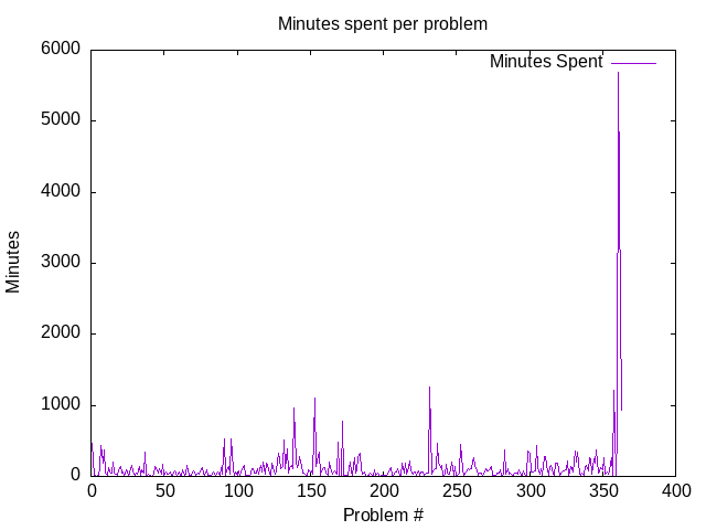
This graph is probably the most representative of the whole problem set. As expected, the last few problems turned out to be among the hardest. The second part of the course turned out to be more time-consuming than the first one.
3.5. Days spent per problem
The figure depicts the number of days (Y-axis) a problem (enumerated by the X-axis coordinate) was loaded in the author’s brain. In simple words, it is the number of days that the state of “trying to solve a problem number X” spanned.
This measure is less justified than the “high concentration” time presented on the figure in the previous section. However, it may nevertheless be useful for encouraging students who get demotivated when spending a long “high concentration” session on a problem with no apparent success. Naturally, most (but not all) problems are solvable within one session (one day).
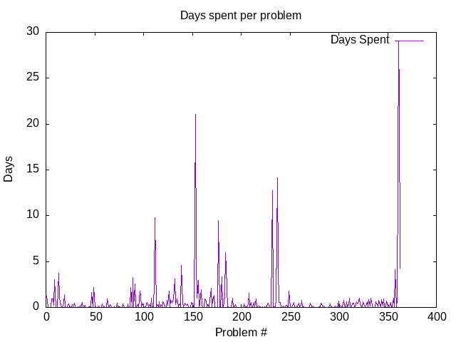
The second spike in the distribution can be attributed to general tiredness while solving such as huge problem set and a need for a break. The corresponding spike on the graph of the study sessions is less prominent.
3.6. Study sessions per problem
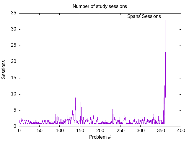
A “session” may be defined as a period of high concentration when the student is actively trying to solve a problem and get the code (or essay) written. This graph presents the number of sessions (Y-axis) spent on each problem (enumerated by the X-axis), regardless of the session length.
When a student goes on a vacation, the problem, presumably, remains loaded in the student’s brain. However, periodic “assaults” in the form of study sessions may be necessary to feed the subconscious processing with the new data.
During vacation time, there should be a spike on the “days per problem” graph, but not the “sessions per problem graph”. This can be seen on the second spike in the “days per problem” graph, which has its counterpart on the “sessions per problem” graph. The counterpart is much shorter.
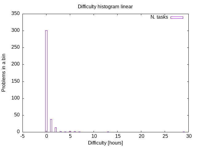
3.7. Difficulty histogram (linear)
The linearly-scaled difficulty histogram depicts how many problems (Y-axis) require up to “bin size” hours for solution. Naturally, most of the exercises are solvable within one to three hours.
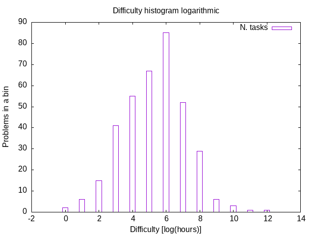
3.8. Difficulty histogram (logarithmic)
The logarithmically-scaled difficulty histogram depicts how many problems (Y-axis) require up to 2\textsuperscript{X} hours for solution. It is very interesting to observe that the histogram shape resembles a uni-modal distribution. It is hard to think of a theoretical foundation on which to base assumptions for the distribution law. Prior research, however, may imply that the distribution is log-normal. (See [10])
4. Conclusion and Further Work
4.1. Conclusion
As follows immediately from the introduction, this report is essentially a single-point estimate of the difficulty distribution of a university-level problem set.
As far as the author knows, this is the first such a complete difficulty breakdown of a university-level problem set in existence.
As has been mentioned in section 3.2, the complete execution of the problem set required 729 hours. In simple words, this is a very long time. If a standard working day is assumed to have the length of 8 hours, the complete solution would require 91 days, or 14 weeks, or 3.5 months.
In the preface to the second edition, the authors claim that a redacted version (e.g. dropping the logical programming part, the part dedicated to the implementation of the register machine simulator, and most of the compiler-related sections) of the course can be covered in one semester. This statement is in agreement with the numbers presented in this report. Nevertheless, as the teachers would probably not want to assign every problem in the book to the student, they would need to make a selection based on both the coverage of the course topics and the time required. The author hopes that this report can provide an insight into the difficulty aspect.
On the other hand, the author would instead recommend opting for a two-semester course. If several of the hardest problems (i.e. problems discussed in section 3.3) are left out, the course can be fitted into two 300-hour modules. Three hundred hours per semester-long course matches the author’s experience of studying partial differential equations at the Moscow Institute of Physics and Technology.
Another important consideration is the amount of time that instructors require to verify solutions and to write feedback for the students. It is reasonable to assume that marking the solutions and writing feedback would require the same amount of time (within an order of magnitude) as the amount needed to solve the problem set, since every problem solution would have to be visited by a marker at least once. For simplicity, the author assumes that writing feedback would require 72 hours per student.
This parameter would then be multiplied by the expected number of students per group, which may vary between institutions, but can be lower-bounded by 5. Therefore the rough estimate would be \(\mbox{const} \cdot 72 \cdot 5 \approx 360\) hours, or 45 full working days (2 months). This duration is hardly practicable for a lone teacher, even if broken down over two semesters. (Each requiring 180 hours.) On the other hand, if the primary teacher is allowed to hire additional staff for marking, the problem becomes manageable again. One of the applications of this report may be as supporting evidence for lead instructors (professors) asking their school administration for teaching assistants.
4.2. Further work
The field of difficulty assessment (especially with the computer-based tools) of university courses still offers a lot to investigate. As far as the author of this report knows, this is the first exhaustive difficulty assessment of a university course. (This is not to say that SICP has not been successfully solved in full before. Various solutions can be found on many well-known software forges.)
The first natural direction of research would then be expanding the same effort towards other problem sets and other subjects.
On the other hand, this report is just a single point estimate, and therefore extremely biased. It may be a significant contribution if the same problem set (or indeed parts or even single problems of it) be solved by different people following the same protocol.
The provision of the solution protocol, the software setup and the time-tracking procedure, is deemed by the author to be a contribution of this report.
Professors teaching such a course are encouraged to show this report to their students and to suggest executing the problem set required along the lines of the protocol given here.
Another research direction could be towards finding an optimal curriculum design beyond the areas covered by SICP. It should not be unexpected if the students decide not to advance further in the course as long as their personal difficulty assessment exceeds a certain unknown threshold. In other words, the author suspects that, at some point, the students may feel an emotion that may be expressed as, “I have been solving this for too long, and see little progress; I should stop.”
It would be interesting to measure such a threshold and to suggest curriculum design strategies that aim to minimise course drop-out. Such strategies may include attempts at hooking into students’ intrinsic motivation (and proper measurements of the execution process may provide an insight on where it is hidden), as well as better designing an extrinsic motivation toolset (e.g. finding better KPIs for rewards and penalties, and proper measures should be helpful in this approach as well).
It would be interesting to observe whether the students who follow the protocol (and see their progress after each session) are more or less likely to drop the course than those who do not. This could constitute a test of intrinsic motivation in line with the self-determination theory of Deci and Ryan (see [32]).
Another important direction may be the development and formalisation of coursework submission formats, in order to facilitate further collection of similar data on this or other problem sets.
4.3. Informal review
This section contains the author’s personal view on the problem set and the questions it raises.
The author (Vladimir Nikishkin), enjoyed doing it. On the other hand, it is hard to believe that teaching this course to first-year undergraduate students can easily be made successful. It is unlikely that a real-world student can dedicate seven hundred hours to a single subject, even if the subject is broken down into two semesters without significant support (the more so, recalling that 25 years has passed since the second edition was released, during which time the world of programming has expanded enormously.) Even if such a student is found, he would probably have other subjects in the semester, as well as the need to attend classes and demonstrations.
Admittedly, out of almost four hundred exercises, the author cannot find a single superfluous one. Even more, the author had to add some extra activities in order to cover several topics better. Every exercise teaches some valuable concept and nudges the student into thinking more deeply.
The course could have been improved in the area of garbage collection and other memory management topics.
Indeed, the main cons-memory garbage collector is explained with sufficient detail to implement it, but several other parts of the interpreter memory model are left without explanation. Very little is said about efficiently storing numbers, strings and other objects.
There is not very much information about a rational process of software development. While this is not fundamental knowledge, but it would be helpful to undergraduates.
The last two exercises amount to one-fifth of the whole work. It was entirely unexpected to see a task to be completed in a language other than Scheme after having already finished most of the exercises.
Probably the biggest drawback of the book is the absence of any conclusion. Indeed, the book points the reader’s attention into various directions by means of an extensive bibliography. However, the author, as a willing student, would like to see a narrativised overview of the possible future directions.
4.4. Informal recommendations
If the author may, by virtue of personally experiencing this transformative experience, give a few suggestions to university curriculum designers, they would be the following:
- Deliberately teach students to use TeX, and especially well technically harnessed TeX (using a professional text editor, additional supportive software, such as syntax checkers, linters, and documentation lookup systems).
This is often considered to be a meta-cognitive exercise to be solved by the students, but the author’s personal experience is not reassuring in this aspect. Very few students, and even professionals, use TeX efficiently. It took more than 50 hours just to refresh the skill of using \TeX{} that the author had already learnt, in order to write a thesis.
- Deliberately teach students to touch-type. This may not be necessary in the regions where touch-typing is included in the standard high school curriculum, but poor touch-typing skills are still a major problem in most parts of the world.
- Deliberately teach students to read software manuals. Indeed, much modern software has manuals built-in piece-wise right into the software itself. Often reading the whole manual is not required to perform the task. However, doing the reading at least once (i.e. reading
somemanual from the first page to the last), is a very enlightening experience, and additionally useful in teaching how to assess the time needed to grasp the skill of usingapiece of software. As a by-product, this experience may help the students to write better manuals for their own software. - Teach students to use a timer when doing homework, even if it is not an org-mode timer. A realistic assessment of how much effort things actually take is a paradigm-shifting experience.
- When writing a book on any subject, start from designing exercises, and afterwards write the text that helps to develop the skills required to solve those. Reading SICP without doing the exercises proved to be almost useless for this project, which was done two years after the first reading.
- Consider introducing elements of industrial illustration standards (UML, ArchiMate) into the teaching flow of an introductory programming course. Courses created to deliberately cover these standards typically suffer from being disconnected from the problem domain. (Few people would like to draw a yet another model of an ATM machine.) Introductory programming provides a surrogate domain that can be mapped onto the diagrams relatively easily and is unlikely to cause rejection.
5. Materials
This section attempts to provide a complete list of materials used in the process of the problem set solution. It is not to be confused with the list of materials used in the preparation of this Experience Report.
5.1. Books
- Structure and Interpretation of Computer Programs 2nd Ed. ([2])
- Structure and Interpretation of Computer Programs 1st Ed. ([1])
- Modern Fortran Explained 2018. ([24])
- Revised\(^7\) Report on Algorithmic Language Scheme. ([34])
- Logic Programming: A Classified Bibliography. ([4])
- Chibi-Scheme Manual. ([33])
- TikZ Manual. ([39])
- PlantUML Manual. ([27])
- UML Weekend Crash Course. ([26])
- GNU Emacs Manual. ([38])
- GNU Emacs Lisp Reference Manual. ([37])
- GNU Emacs Org-Mode Manual. ([11])
- Debugging With GDB. ([36])
- Implementations of Prolog. ([6])
5.2. Software
5.3. Papers
- Revised Report on the Propagator Model. ([30])
- On Implementing Prolog In Functional Programming. ([8])
- eu-Prolog, Reference Manual. ([20])
References
| [1] | Harold Abelson and Gerald J. Sussman. Structure and Interpretation of Computer Programs. MIT Press, 1 edition, 1985. [ bib ] |
| [2] | Harold Abelson, Gerald J. Sussman, and Julia Sussman. Structure and Interpretation of Computer Programs. MIT Press, 2 edition, 1996. [ bib ] |
| [3] | Dan L. Adler and Jacob S. Kounin. Some factors operating at the moment of resumption of interrupted tasks. 7(2):255--267. [ bib | DOI | http ] |
| [4] | Isaac Balbin and Koenraad Lecot. Logic Programming. Springer Netherlands, 1985. [ bib | DOI | http ] |
| [5] | Eric Berne. What Do You Say After You Say Hello? Bantam Books, New York, 1973. [ bib ] |
| [6] | John A. Campbell, editor. Implementations of Prolog. Ellis Horwood/Halsted Press/Wiley, 1984. [ bib ] |
| [7] | Taylor Campbell et al. MIT/GNU Scheme, 2019. [ bib | http ] |
| [8] | Mats Carlsson. On implementing Prolog in functional programming. 2(4):347--359, 1984. [ bib | DOI | http ] |
| [9] | Karen L. St. Clair. A case against compulsory class attendance policies in higher education. 23(3):171--180, 1999. [ bib | DOI | http ] |
| [10] | Edwin L. Crow and Kunio Shimizu. Lognormal Distributions: Theory and Applications. Routledge, 5 2018. [ bib | DOI | http ] |
| [11] | Carsten Dominik. The Org-Mode 7 Reference Manual: Organize Your Life with GNU Emacs. Network Theory, UK, 2010. with contributions by David O'Toole, Bastien Guerry, Philip Rooke, Dan Davison, Eric Schulte, and Thomas Dye. [ bib ] |
| [12] | Carsten Dominik et al. Org-mode, 2019. [ bib | http ] |
| [13] | John Ellson et al. Graphviz. [ bib | http ] |
| [14] | Matthias Felleisen, Robert Bruce Findler, Matthew Flatt, and Shriram Krishnamurthi. The structure and interpretation of the computer science curriculum. 14:365--378, 07 2004. [ bib | DOI ] |
| [15] | Matthias Felleisen, Robert Bruce Findler, Matthew Flatt, and Shriram Krishnamurthi. How to Design Programs: an Introduction to Programming and Computing. The MIT Press, Cambridge, Massachusetts, 2018. [ bib ] |
| [16] | Free Software Foundation. GNU Emacs, 2019. [ bib | http ] |
| [17] | Free Software Foundation. GNU debugger, 2020. [ bib | http ] |
| [18] | Floyd W. Gembicki and Yacov Y. Haimes. Approach to performance and sensitivity multiobjective optimization: The goal attainment method. 20(6):769--771, December 1975. [ bib | DOI | http ] |
| [19] | Martin Hlosta, Drahomira Herrmannova, Lucie Vachova, Jakub Kuzilek, Zdenek Zdrahal, and Annika Wolff. Modelling student online behaviour in a virtual learning environment. 2018. [ bib ] |
| [20] | Eugene Kohlbecker. eu-Prolog, reference manual and report. Technical report, University of Indiana (Bloomington), Computer Science Department, 04 1984. [ bib ] |
| [21] | E. W. Kooker. Changes in grade distributions associated with changes in class attendance policies. 13:56--57, 1976. [ bib ] |
| [22] | Kelly Y. L. Ku and Irene T. Ho. Metacognitive strategies that enhance critical thinking. 5(3):251--267, July 2010. [ bib | DOI | http ] |
| [23] | Douglas McGregor. Theory X and theory Y. 358:374, 1960. [ bib ] |
| [24] | Michael Metcalf, John Reid, and Malcolm Cohen. Modern Fortran Explained. Oxford University Press, 10 2018. [ bib | DOI | http ] |
| [25] | Vladimir Nikishkin. A full solution to the structure and interpretation of computer programs. [ bib | http ] |
| [26] | Thomas Pender. UML Weekend Crash Course. Hungry Minds, Indianapolis, IN, 2002. [ bib ] |
| [27] | PlantUML Developers. Drawing UML with plantuml. [ bib | http ] |
| [28] | PlantUML Developers. PlantUML. [ bib | http ] |
| [29] | Project Jupyter Developers. Jupyter Notebook: a server-client application that allows editing and running notebook documents via a web browser., 2019. [ bib | http ] |
| [30] | Alexey Radul and Gerald J. Sussman. Revised report on the propagator model. [ bib | http ] |
| [31] | Jose A. O. Ruiz et al. geiser, 2020. [ bib | .html ] |
| [32] | Richard M Ryan and Edward L Deci. Self-determination theory: Basic psychological needs in motivation, development, and wellness. Guilford Publications, 2017. [ bib ] |
| [33] | Alex Shinn. Chibi-Scheme. [ bib | http ] |
| [34] | Alex Shinn, John Cowan, Arthur A. Gleckler, et al., editors. Revised7 Report on the Algorithmic Language Scheme. 2013. [ bib | http ] |
| [35] | Alex Shinn et al. Chibi-Scheme, 2019. [ bib | http ] |
| [36] | Richard Stallman et al. Debugging with GDB, 2020. [ bib | .html ] |
| [37] | Richard Stallman et al. GNU Emacs Lisp Reference Manual, 2020. [ bib | .pdf ] |
| [38] | Richard Stallman et al. GNU Emacs Manual, 2020. [ bib | .pdf ] |
| [39] | Till Tantau. The TikZ and PGF Packages. [ bib | .pdf ] |
| [40] | Till Tantau et al. Portable graphics format. [ bib | http ] |
| [41] | TeX User Groups. TeX Live, 2019. [ bib | http ] |
| [42] | Jeffrey J. VanWormer, Simone A. French, Mark A. Pereira, and Ericka M. Welsh. The impact of regular self-weighing on weight management: A systematic literature review. 5(1):54, 2008. [ bib | DOI | http ] |
| [43] | Patric Volkerding et al. Slackware Linux, 2019. [ bib | http ] |
6. Appendix: Analysed data on problem difficulty
For the code used to generate the tables in the following sections, see: Appendix: Emacs Lisp code for data analysis.
6.1. Analysed time consumption
| No | Exercise Name | Days Spent | Spans Sessions | Minutes Spent |
|---|---|---|---|---|
| 1 | Exercise 1.1 Interpreter result | 1.211 | 2 | 459 |
| 2 | Exercise 1.2 Prefix form | 0.001 | 1 | 2 |
| 3 | Figure 1.1 Tree representation, showing the value of each su | 0.007 | 1 | 10 |
| 4 | Exercise 1.4 Compound expressions | 0.003 | 1 | 4 |
| 5 | Exercise 1.5 Ben’s test | 0.008 | 1 | 11 |
| 6 | Exercise 1.6 If is a special form | 0.969 | 2 | 118 |
| 7 | Exercise 1.7 Good enough? | 0.949 | 3 | 436 |
| 8 | Exercise 1.8 Newton’s method | 0.197 | 2 | 193 |
| 9 | Exercise 1.10 Ackermann’s function | 3.038 | 2 | 379 |
| 10 | Exercise 1.11 Recursive vs iterative | 0.037 | 1 | 54 |
| 11 | Exercise 1.12 Recursive Pascal’s triangle | 0.012 | 1 | 17 |
| 12 | Exercise 1.13 Fibonacci | 0.092 | 1 | 132 |
| 13 | Exercise 1.9 Iterative or recursive? | 3.722 | 2 | 65 |
| 14 | Exercise 1.14 count-change | 1.038 | 2 | 50 |
| 15 | Exercise 1.15 sine | 0.267 | 2 | 195 |
| 16 | Exercise 1.16 Iterative exponentiation | 0.032 | 1 | 46 |
| 17 | Exercise 1.17 Fast multiplication | 0.019 | 1 | 28 |
| 18 | Exercise 1.18 Iterative multiplication | 0.497 | 2 | 23 |
| 19 | Exercise 1.19 Logarithmic Fibonacci | 1.374 | 2 | 93 |
| 20 | Exercise 1.20 GCD applicative vs normal | 0.099 | 1 | 142 |
| 21 | Exercise 1.21 smallest-divisor | 0.027 | 1 | 39 |
| 22 | Exercise 1.22 timed-prime-test | 0.042 | 1 | 61 |
| 23 | Exercise 1.23 (next test-divisor) | 0.383 | 2 | 5 |
| 24 | Exercise 1.24 Fermat method | 0.067 | 1 | 96 |
| 25 | Exercise 1.25 expmod | 0.051 | 1 | 74 |
| 26 | Exercise 1.26 square vs mul | 0.003 | 1 | 4 |
| 27 | Exercise 1.27 Carmichael numbers | 0.333 | 2 | 102 |
| 28 | Exercise 1.28 Miller-Rabin | 0.110 | 1 | 158 |
| 29 | Exercise 1.29 Simpson’s integral | 0.464 | 2 | 68 |
| 30 | Exercise 1.30 Iterative sum | 0.030 | 2 | 10 |
| 31 | Exercise 1.31 Product | 0.028 | 1 | 40 |
| 32 | Exercise 1.32 Accumulator | 0.017 | 1 | 24 |
| 33 | Exercise 1.33 filtered-accumulate | 0.092 | 1 | 133 |
| 34 | Exercise 1.34 lambda | 0.006 | 1 | 8 |
| 35 | Exercise 1.35 fixed-point | 0.265 | 2 | 87 |
| 36 | Exercise 1.36 fixed-point-with-dampening | 0.035 | 1 | 50 |
| 37 | Exercise 1.37 cont-frac | 0.569 | 2 | 348 |
| 38 | Exercise 1.38 euler constant | 0.000 | 1 | 0 |
| 39 | Exercise 1.39 tan-cf | 0.025 | 1 | 36 |
| 40 | Exercise 1.40 newtons-method | 0.205 | 2 | 6 |
| 41 | Exercise 1.41 double-double | 0.010 | 1 | 15 |
| 42 | Exercise 1.42 compose | 0.004 | 1 | 6 |
| 43 | Exercise 1.43 repeated | 0.019 | 1 | 27 |
| 44 | Exercise 1.44 smoothing | 0.099 | 2 | 142 |
| 45 | Exercise 1.45 nth-root | 0.056 | 1 | 80 |
| 46 | Exercise 1.46 iterative-improve | 0.033 | 1 | 48 |
| 47 | Exercise 2.1 make-rat | 1.608 | 2 | 109 |
| 48 | Exercise 2.2 make-segment | 0.024 | 1 | 34 |
| 49 | Exercise 2.3 make-rectangle | 2.183 | 2 | 174 |
| 50 | Exercise 2.4 cons-lambda | 0.007 | 1 | 10 |
| 51 | Exercise 2.5 cons-pow | 0.041 | 1 | 59 |
| 52 | Exercise 2.6 Church Numerals | 0.024 | 1 | 34 |
| 53 | Exercise 2.7 make-interval | 0.019 | 1 | 28 |
| 54 | Exercise 2.8 sub-interval | 0.124 | 1 | 58 |
| 55 | Exercise 2.9 interval-width | 0.006 | 1 | 8 |
| 56 | Exercise 2.10 div-interval-better | 0.010 | 1 | 15 |
| 57 | Exercise 2.11 mul-interval-nine-cases | 0.052 | 1 | 75 |
| 58 | Exercise 2.12 make-center-percent | 0.393 | 2 | 43 |
| 59 | Exercise 2.13 formula for tolerance | 0.003 | 1 | 5 |
| 60 | Exercise 2.14 parallel-resistors | 0.047 | 1 | 68 |
| 61 | Exercise 2.15 better-intervals | 0.007 | 1 | 10 |
| 62 | Exercise 2.16 interval-arithmetic | 0.002 | 1 | 3 |
| 63 | Exercise 2.17 last-pair | 0.966 | 2 | 89 |
| 64 | Exercise 2.18 reverse | 0.006 | 1 | 9 |
| 65 | Exercise 2.19 coin-values | 0.021 | 1 | 30 |
| 66 | Exercise 2.20 dotted-tail notation | 0.311 | 2 | 156 |
| 67 | Exercise 2.21 map-square-list | 0.013 | 1 | 19 |
| 68 | Exercise 2.22 wrong list order | 0.007 | 1 | 10 |
| 69 | Exercise 2.23 for-each | 0.006 | 1 | 9 |
| 70 | Exercise 2.24 list-plot-result | 0.111 | 2 | 75 |
| 71 | Exercise 2.25 caddr | 0.037 | 1 | 54 |
| 72 | Exercise 2.26 append cons list | 0.011 | 1 | 16 |
| 73 | Exercise 2.27 deep-reverse | 0.433 | 2 | 40 |
| 74 | Exercise 2.28 fringe | 0.026 | 1 | 37 |
| 75 | Exercise 2.29 mobile | 0.058 | 1 | 83 |
| 76 | Exercise 2.30 square-tree | 0.100 | 2 | 122 |
| 77 | Exercise 2.31 tree-map square tree | 0.019 | 1 | 27 |
| 78 | Exercise 2.32 subsets | 0.010 | 1 | 15 |
| 79 | Exercise 2.33 map-append-length | 0.375 | 2 | 96 |
| 80 | Exercise 2.34 horners-rule | 0.006 | 1 | 8 |
| 81 | Exercise 2.35 count-leaves-accumulate | 0.011 | 1 | 16 |
| 82 | Exercise 2.36 accumulate-n | 0.006 | 1 | 9 |
| 83 | Exercise 2.37 matrix-*-vector | 0.017 | 1 | 24 |
| 84 | Exercise 2.38 fold-left | 0.372 | 2 | 65 |
| 85 | Exercise 2.39 reverse fold-right fold-left | 0.005 | 1 | 7 |
| 86 | Exercise 2.40 unique-pairs | 0.029 | 1 | 42 |
| 87 | Exercise 2.41 triple-sum | 2.195 | 2 | 57 |
| 88 | Figure 2.8 A solution to the eight-queens puzzle. | 0.001 | 1 | 2 |
| 89 | Exercise 2.42 k-queens | 3.299 | 2 | 122 |
| 90 | Exercise 2.43 slow k-queens | 0.019 | 1 | 28 |
| 91 | Exercise 2.46 make-vect | 2.578 | 5 | 535 |
| 92 | Exercise 2.47 make-frame | 0.083 | 1 | 10 |
| 93 | Exercise 2.48 make-segment | 0.054 | 1 | 78 |
| 94 | Exercise 2.49 segments->painter applications | 0.294 | 2 | 139 |
| 95 | Exercise 2.50 flip-horiz and rotate270 and rotate180 | 0.019 | 1 | 27 |
| 96 | Exercise 2.51 below | 1.801 | 4 | 524 |
| 97 | Exercise 2.44 up-split | 1.169 | 2 | 89 |
| 98 | Exercise 2.45 split | 0.113 | 2 | 23 |
| 99 | Exercise 2.52 modify square-limit | 0.450 | 2 | 58 |
| 100 | Exercise 2.53 quote introduction | 0.008 | 1 | 11 |
| 101 | Exercise 2.54 equal? implementation | 0.050 | 1 | 72 |
| 102 | Exercise 2.55 quote quote | 0.000 | 1 | 0 |
| 103 | Exercise 2.56 differentiation-exponentiation | 0.393 | 2 | 65 |
| 104 | Exercise 2.57 differentiate-three-sum | 0.560 | 3 | 147 |
| 105 | Exercise 2.58 infix-notation | 0.112 | 1 | 161 |
| 106 | Exercise 2.59 union-set | 0.277 | 2 | 6 |
| 107 | Exercise 2.60 duplicate-set | 0.012 | 1 | 17 |
| 108 | Exercise 2.62 ordered-union-set (ordered list) | 0.973 | 2 | 14 |
| 109 | Exercise 2.61 sets as ordered lists | 0.004 | 1 | 6 |
| 110 | Exercise 2.63 tree->list (binary search tree) | 0.078 | 1 | 113 |
| 111 | Exercise 2.64 balanced-tree | 2.740 | 3 | 106 |
| 112 | Exercise 2.65 tree-union-set | 9.785 | 2 | 47 |
| 113 | Exercise 2.66 tree-lookup | 0.035 | 1 | 50 |
| 114 | Exercise 2.67 Huffman decode a simple message | 0.303 | 3 | 108 |
| 115 | Exercise 2.68 Huffman encode a simple message | 0.023 | 1 | 33 |
| 116 | Exercise 2.69 Generate Huffman tree | 0.608 | 2 | 160 |
| 117 | Exercise 2.70 Generate a tree and encode a song | 0.072 | 2 | 57 |
| 118 | Exercise 2.71 Huffman tree for frequencies 5 and 10 | 0.258 | 2 | 202 |
| 119 | Exercise 2.72 Huffman order of growth | 0.050 | 2 | 26 |
| 120 | Exercise 2.73 data-driven-deriv | 0.605 | 2 | 189 |
| 121 | Exercise 2.74 Insatiable Enterprises | 0.410 | 4 | 171 |
| 122 | Exercise 2.75 make-from-mag-ang message passing | 0.019 | 1 | 28 |
| 123 | Exercise 2.76 types or functions? | 0.003 | 1 | 5 |
| 124 | Exercise 2.77 generic-algebra-magnitude | 0.772 | 3 | 190 |
| 125 | Exercise 2.78 Ordinary numbers for Scheme | 0.212 | 2 | 67 |
| 126 | Exercise 2.79 generic-equality | 1.786 | 2 | 28 |
| 127 | Exercise 2.80 Generic arithmetic zero? | 0.056 | 1 | 80 |
| 128 | Exercise 2.81 coercion to-itself | 0.749 | 3 | 330 |
| 129 | Exercise 2.82 three-argument-coercion | 0.433 | 2 | 230 |
| 130 | Exercise 2.83 Numeric Tower and (raise) | 0.717 | 3 | 116 |
| 131 | Exercise 2.84 Using raise (raise-type) in apply-generic |
0.865 | 2 | 135 |
| 132 | Exercise 2.85 Dropping a type | 3.089 | 5 | 507 |
| 133 | Exercise 2.86 Compound complex numbers | 0.274 | 2 | 108 |
| 134 | Exercise 2.87 Generalized zero? | 0.919 | 4 | 389 |
| 135 | Exercise 2.88 Subtraction of polynomials | 0.646 | 3 | 50 |
| 136 | Exercise 2.89 Dense term-lists | 0.083 | 1 | 120 |
| 137 | Exercise 2.90 Implementing dense polynomials as a separate p | 0.400 | 2 | 148 |
| 138 | Exercise 2.91 Division of polynomials | 0.111 | 2 | 103 |
| 139 | Exercise 2.92 Ordering of variables so that addition and mul | 4.556 | 11 | 964 |
| 140 | Exercise 2.93 Rational polynomials | 0.378 | 3 | 198 |
| 141 | Exercise 2.94 Greatest-common-divisor for polynomials | 0.091 | 1 | 131 |
| 142 | Exercise 2.95 Illustrate the non-integer problem | 0.450 | 2 | 149 |
| 143 | Exercise 2.96 Integerizing factor | 0.325 | 2 | 275 |
| 144 | Exercise 2.97 Reduction of polynomials | 0.201 | 1 | 140 |
| 145 | Exercise 3.1 accumulators | 0.425 | 2 | 53 |
| 146 | Exercise 3.2 make-monitored | 0.027 | 1 | 39 |
| 147 | Exercise 3.3 password protection | 0.010 | 1 | 14 |
| 148 | Exercise 3.4 call-the-cops | 0.010 | 1 | 15 |
| 149 | Exercise 3.5 Monte-Carlo | 0.528 | 2 | 98 |
| 150 | Exercise 3.6 reset a prng | 0.479 | 2 | 68 |
| 151 | Exercise 3.7 Joint accounts | 0.059 | 1 | 85 |
| 152 | Exercise 3.8 Right-to-left vs Left-to-right | 0.026 | 1 | 38 |
| 153 | Exercise 3.9 Environment structures | 21.030 | 10 | 1100 |
| 154 | Exercise 3.10 Using let to create state variables |
4.933 | 2 | 138 |
| 155 | Exercise 3.11 Internal definitions | 0.994 | 2 | 219 |
| 156 | Exercise 3.12 Drawing append! |
2.966 | 3 | 347 |
| 157 | Exercise 3.13 make-cycle |
0.010 | 1 | 14 |
| 158 | Exercise 3.14 mystery |
0.385 | 2 | 77 |
| 159 | Exercise 3.15 set-to-wow! |
1.942 | 3 | 117 |
| 160 | Exercise 3.16 count-pairs |
0.171 | 1 | 118 |
| 161 | Exercise 3.17 Real count-pairs |
0.029 | 1 | 42 |
| 162 | Exercise 3.18 Finding cycles | 0.012 | 1 | 17 |
| 163 | Exercise 3.19 Efficient finding cycles | 0.934 | 2 | 205 |
| 164 | Exercise 3.20 Procedural set-car! |
0.633 | 2 | 121 |
| 165 | Exercise 3.21 queues | 0.021 | 1 | 30 |
| 166 | Exercise 3.22 procedural queue | 0.294 | 2 | 67 |
| 167 | Exercise 3.23 dequeue | 0.049 | 2 | 71 |
| 168 | Exercise 3.24 tolerant tables | 0.780 | 3 | 33 |
| 169 | Exercise 3.25 multilevel tables | 2.103 | 2 | 486 |
| 170 | Exercise 3.26 binary tree table | 0.013 | 1 | 18 |
| 171 | Exercise 3.27 memoization | 0.802 | 2 | 2 |
| 172 | Exercise 3.28 primitive or-gate | 1.316 | 2 | 783 |
| 173 | Exercise 3.29 Compound or-gate | 0.001 | 1 | 2 |
| 174 | Exercise 3.30 ripple-carry adder | 0.009 | 1 | 13 |
| 175 | Exercise 3.31 Initial propagation | 0.013 | 1 | 18 |
| 176 | Exercise 3.32 Order matters | 0.007 | 1 | 10 |
| 177 | Exercise 3.33 averager constraint | 9.460 | 3 | 198 |
| 178 | Exercise 3.34 Wrong squarer | 0.042 | 1 | 61 |
| 179 | Exercise 3.35 Correct squarer | 0.012 | 1 | 17 |
| 180 | Exercise 3.36 Connector environment diagram | 3.319 | 3 | 263 |
| 181 | Exercise 3.37 Expression-based constraints | 0.037 | 1 | 53 |
| 182 | Exercise 3.38 Timing | 0.061 | 1 | 88 |
| 183 | Exercise 3.39 Serializer | 1.266 | 4 | 269 |
| 184 | Exercise 3.40 Three parallel multiplications | 5.973 | 3 | 332 |
| 185 | Exercise 3.41 Better protected account | 4.229 | 2 | 97 |
| 186 | Exercise 3.42 Saving on serializers | 0.023 | 1 | 33 |
| 187 | Exercise 3.43 Multiple serializations | 0.040 | 1 | 58 |
| 188 | Exercise 3.44 Transfer money | 0.005 | 1 | 7 |
| 189 | Exercise 3.45 new plus old serializers | 0.004 | 1 | 6 |
| 190 | Exercise 3.46 broken test-and-set! | 0.007 | 1 | 10 |
| 191 | Exercise 3.47 semaphores | 1.044 | 2 | 53 |
| 192 | Exercise 3.48 serialized-exchange deadlock | 0.022 | 1 | 31 |
| 193 | Exercise 3.49 When numbering accounts doesn’t work | 0.008 | 1 | 11 |
| 194 | Exercise 3.50 stream-map multiple arguments | 0.317 | 3 | 96 |
| 195 | Exercise 3.51 stream-show | 0.007 | 1 | 10 |
| 196 | Exercise 3.52 streams with mind-boggling | 0.034 | 1 | 49 |
| 197 | Exercise 3.53 stream power of two | 0.016 | 1 | 23 |
| 198 | Exercise 3.54 mul-streams | 0.005 | 1 | 7 |
| 199 | Exercise 3.55 streams partial-sums | 0.013 | 1 | 18 |
| 200 | Exercise 3.56 Hamming’s streams-merge | 0.015 | 1 | 21 |
| 201 | Exercise 3.57 exponential additions fibs | 0.007 | 1 | 10 |
| 202 | Exercise 3.58 Cryptic stream | 0.010 | 1 | 14 |
| 203 | Exercise 3.59 power series | 0.422 | 2 | 30 |
| 204 | Exercise 3.60 mul-series | 0.048 | 1 | 69 |
| 205 | Exercise 3.61 power-series-inversion | 0.087 | 1 | 126 |
| 206 | Exercise 3.62 div-series | 0.006 | 1 | 8 |
| 207 | Exercise 3.63 sqrt-stream | 0.299 | 2 | 8 |
| 208 | Exercise 3.64 stream-limit | 1.546 | 2 | 55 |
| 209 | Exercise 3.65 approximating logarithm | 0.039 | 1 | 56 |
| 210 | Exercise 3.66 lazy pairs | 0.515 | 2 | 107 |
| 211 | Exercise 3.67 all possible pairs | 0.010 | 1 | 14 |
| 212 | Exercise 3.68 pairs-louis | 0.012 | 1 | 17 |
| 213 | Exercise 3.70 merge-weighted | 0.522 | 2 | 188 |
| 214 | Exercise 3.71 Ramanujan numbers | 0.035 | 1 | 51 |
| 215 | Exercise 3.72 Ramanujan 3-numbers | 0.901 | 2 | 187 |
| 216 | Figure 3.32 | 0.022 | 1 | 32 |
| 217 | Exercise 3.73 RC-circuit | 0.090 | 1 | 130 |
| 218 | Exercise 3.74 zero-crossings | 0.153 | 1 | 221 |
| 219 | Exercise 3.75 filtering signals | 0.056 | 1 | 81 |
| 220 | Exercise 3.76 stream-smooth | 0.073 | 2 | 36 |
| 221 | Exercise 3.77 | 0.038 | 1 | 55 |
| 222 | Exercise 3.78 second order differential equation | 0.039 | 1 | 56 |
| 223 | Exercise 3.79 general second-order ode | 0.007 | 1 | 10 |
| 224 | Figure 3.36 | 0.058 | 1 | 84 |
| 225 | Exercise 3.80 RLC circuit | 0.013 | 1 | 19 |
| 226 | Exercise 3.81 renerator-in-streams | 0.040 | 1 | 57 |
| 227 | Exercise 3.82 streams Monte-Carlo | 0.378 | 2 | 57 |
| 228 | Exercise 4.1 list-of-values ordered | 0.437 | 2 | 14 |
| 229 | Exercise 4.2 application before assignments | 0.021 | 1 | 30 |
| 230 | Exercise 4.3 data-directed eval | 0.030 | 1 | 43 |
| 231 | Exercise 4.4 eval-and and eval-or | 0.035 | 1 | 50 |
| 232 | Exercise 4.5 cond with arrow | 12.765 | 7 | 1252 |
| 233 | Exercise 4.6 Implementing let | 0.019 | 1 | 27 |
| 234 | Exercise 4.7 Implementing let* | 0.046 | 1 | 66 |
| 235 | Exercise 4.8 Implementing named let | 0.070 | 1 | 101 |
| 236 | Exercise 4.9 Implementing until | 0.928 | 3 | 102 |
| 237 | Exercise 4.10 Modifying syntax | 14.168 | 3 | 462 |
| 238 | Exercise 4.11 Environment as a list of bindings | 4.368 | 2 | 194 |
| 239 | Exercise 4.12 Better abstractions for setting a value | 0.529 | 2 | 120 |
| 240 | Exercise 4.13 Implementing make-unbound! |
0.550 | 2 | 149 |
| 241 | Exercise 4.14 meta map versus built-in map | 0.004 | 1 | 6 |
| 242 | Exercise 4.15 The halts? predicate |
0.018 | 1 | 26 |
| 243 | Exercise 4.16 Simultaneous internal definitions | 0.162 | 2 | 177 |
| 244 | Exercise 4.17 Environment with simultaneous definitions | 0.036 | 1 | 52 |
| 245 | Exercise 4.18 Alternative scanning | 0.018 | 1 | 26 |
| 246 | Exercise 4.19 Mutual simultaneous definitions | 0.220 | 2 | 96 |
| 247 | Exercise 4.20 letrec | 0.206 | 2 | 195 |
| 248 | Exercise 4.21 Y-combinator | 0.013 | 1 | 18 |
| 249 | Exercise 4.22 Extending evaluator to support let |
1.768 | 3 | 144 |
| 250 | Exercise 4.23 Analysing sequences | 0.005 | 1 | 7 |
| 251 | Exercise 4.24 Analysis time test | 0.022 | 1 | 32 |
| 252 | Exercise 4.25 lazy factorial | 0.034 | 1 | 49 |
| 253 | Exercise 4.26 unless as a special form | 0.313 | 1 | 451 |
| 254 | Exercise 4.27 Working with mutation in lazy interpreters | 0.515 | 2 | 112 |
| 255 | Exercise 4.28 Eval before applying | 0.005 | 1 | 7 |
| 256 | Exercise 4.29 Lazy evaluation is slow without memoization | 0.035 | 1 | 50 |
| 257 | Exercise 4.30 Lazy sequences | 0.153 | 2 | 74 |
| 258 | Exercise 4.31 Lazy arguments with syntax extension | 0.092 | 2 | 112 |
| 259 | Exercise 4.32 streams versus lazy lists | 0.503 | 2 | 87 |
| 260 | Exercise 4.33 quoted lazy lists | 0.097 | 2 | 103 |
| 261 | Exercise 4.34 printing lazy lists | 0.219 | 3 | 205 |
| 262 | Exercise 4.50 The ramb operator |
0.813 | 4 | 266 |
| 263 | Exercise 4.35 an-integer-between and Pythagorean triples |
0.103 | 2 | 138 |
| 264 | Exercise 3.69 triples | 0.115 | 2 | 85 |
| 265 | Exercise 4.36 infinite search for Pythagorean triples | 0.011 | 1 | 16 |
| 266 | Exercise 4.37 another method for triples | 0.035 | 1 | 51 |
| 267 | Exercise 4.38 Logical puzzle - Not same floor | 0.027 | 1 | 39 |
| 268 | Exercise 4.39 Order of restrictions | 0.003 | 1 | 5 |
| 269 | Exercise 4.40 People to floor assignment | 0.019 | 1 | 28 |
| 270 | Exercise 4.41 Ordinary Scheme to solve the problem | 0.072 | 1 | 103 |
| 271 | Exercise 4.42 The liars puzzle | 0.503 | 1 | 81 |
| 272 | Exercise 4.43 Problematical Recreations | 0.052 | 1 | 75 |
| 273 | Exercise 4.44 Nondeterministic eight queens | 0.074 | 1 | 106 |
| 274 | Exercise 4.45 Five parses | 0.186 | 3 | 145 |
| 275 | Exercise 4.46 Order of parsing | 0.007 | 1 | 10 |
| 276 | Exercise 4.47 Parse verb phrase by Louis | 0.013 | 1 | 18 |
| 277 | Exercise 4.48 Extending the grammar | 0.037 | 1 | 1 |
| 278 | Exercise 4.49 Alyssa’s generator | 0.031 | 1 | 45 |
| 279 | Exercise 4.51 Implementing permanent-set! |
0.030 | 1 | 43 |
| 280 | Exercise 4.52 if-fail |
0.063 | 1 | 91 |
| 281 | Exercise 4.53 test evaluation | 0.005 | 1 | 7 |
| 282 | Exercise 4.54 analyze-require |
0.468 | 2 | 31 |
| 283 | Exercise 4.55 Simple queries | 0.258 | 2 | 372 |
| 284 | Exercise 4.56 Compound queries | 0.018 | 1 | 26 |
| 285 | Exercise 4.57 custom rules | 0.147 | 3 | 112 |
| 286 | Exercise 4.58 big shot | 0.025 | 1 | 36 |
| 287 | Exercise 4.59 meetings | 0.031 | 1 | 45 |
| 288 | Exercise 4.60 pairs live near | 0.016 | 1 | 23 |
| 289 | Exercise 4.61 next-to relation | 0.008 | 1 | 11 |
| 290 | Exercise 4.62 last-pair | 0.033 | 1 | 48 |
| 291 | Exercise 4.63 Genesis | 0.423 | 2 | 40 |
| 292 | Figure 4.6 How the system works | 0.022 | 1 | 31 |
| 293 | Exercise 4.64 broken outranked-by | 0.065 | 1 | 94 |
| 294 | Exercise 4.65 second-degree subordinates | 0.012 | 1 | 17 |
| 295 | Exercise 4.66 Ben’s accumulation | 0.013 | 1 | 18 |
| 296 | Exercise 4.70 Cons-stream delays its second argument | 0.167 | 3 | 79 |
| 297 | Exercise 4.72 interleave-stream | 0.002 | 1 | 3 |
| 298 | Exercise 4.73 flatten-stream delays | 0.006 | 1 | 8 |
| 299 | Exercise 4.67 loop detector | 0.251 | 1 | 361 |
| 300 | Exercise 4.68 reverse rule | 0.686 | 2 | 321 |
| 301 | Exercise 4.69 great grandchildren | 0.080 | 2 | 65 |
| 302 | Exercise 4.71 Louis’ simple queries | 0.134 | 2 | 69 |
| 303 | Exercise 4.74 Alyssa’s streams | 0.044 | 1 | 64 |
| 304 | Exercise 4.75 unique special form |
0.055 | 1 | 79 |
| 305 | Exercise 4.76 improving and |
0.797 | 2 | 438 |
| 306 | Figure 5.2 Controller for a GCD Machine | 0.167 | 3 | 124 |
| 307 | Exercise 5.1 Register machine plot | 0.020 | 1 | 29 |
| 308 | Figure 5.1 Data paths for a Register Machine | 0.599 | 2 | 115 |
| 309 | Exercise 5.2 Register machine language description of Exerci | 0.006 | 1 | 8 |
| 310 | Exercise 5.3 Machine for sqrt using Newton Method |
0.306 | 2 | 286 |
| 311 | Exercise 5.4 Recursive register machines | 1.001 | 4 | 274 |
| 312 | Exercise 5.5 Hand simulation for factorial and Fibonacci | 0.110 | 1 | 158 |
| 313 | Exercise 5.6 Fibonacci machine extra instructions | 0.011 | 1 | 16 |
| 314 | Exercise 5.7 Test the 5.4 machine on a simulator | 0.458 | 2 | 133 |
| 315 | Exercise 5.8 Ambiguous labels | 0.469 | 1 | 160 |
| 316 | Exercise 5.9 Prohibit (op)s on labels | 0.017 | 1 | 25 |
| 317 | Exercise 5.10 Changing syntax | 0.011 | 1 | 16 |
| 318 | Exercise 5.11 Save and restore | 0.619 | 3 | 186 |
| 319 | Exercise 5.12 Data paths from controller | 0.424 | 2 | 183 |
| 320 | Exercise 5.13 Registers from controller | 0.470 | 2 | 101 |
| 321 | Exercise 1.3 Sum of squares | 1.044 | 1 | 6 |
| 322 | Exercise 5.14 Profiling | 0.347 | 2 | 57 |
| 323 | Exercise 5.15 Instruction counting | 0.052 | 1 | 75 |
| 324 | Exercise 5.16 Tracing execution | 0.058 | 1 | 83 |
| 325 | Exercise 5.18 Register tracing | 0.631 | 2 | 90 |
| 326 | Exercise 5.19 Breakpoints | 0.149 | 1 | 215 |
| 327 | Exercise 5.17 Printing labels | 0.001 | 1 | 1 |
| 328 | Exercise 5.20 Drawing a list “(#1=(1 . 2) #1)” |
0.189 | 2 | 139 |
| 329 | Exercise 5.21 Register machines for list operations | 0.617 | 2 | 115 |
| 330 | Exercise 5.22 append and append! as register machines |
0.047 | 1 | 68 |
| 331 | Exercise 5.23 Extending EC-evaluator with let and cond |
0.862 | 4 | 363 |
| 332 | Exercise 5.24 Making cond a primitive |
0.160 | 2 | 199 |
| 333 | Exercise 5.25 Normal-order (lazy) evaluation | 1.010 | 4 | 342 |
| 334 | Exercise 5.26 Explore tail recursion with factorial |
0.195 | 2 | 26 |
| 335 | Exercise 5.27 Stack depth for a recursive factorial | 0.008 | 1 | 11 |
| 336 | Exercise 5.28 Interpreters without tail recursion | 0.028 | 1 | 40 |
| 337 | Exercise 5.29 Stack in tree-recursive Fibonacci | 0.015 | 1 | 21 |
| 338 | Exercise 5.30 Errors | 0.615 | 3 | 147 |
| 339 | Exercise 5.31 a preserving mechanism |
0.417 | 2 | 161 |
| 340 | Exercise 5.32 symbol-lookup optimization | 0.052 | 1 | 75 |
| 341 | Exercise 5.33 compiling factorial-alt |
0.753 | 2 | 267 |
| 342 | Exercise 5.34 compiling iterative factorial | 0.169 | 1 | 243 |
| 343 | Exercise 5.35 Decompilation | 0.022 | 1 | 32 |
| 344 | Exercise 5.36 Order of evaluation | 0.845 | 4 | 256 |
| 345 | Exercise 5.37 preserving |
0.135 | 1 | 194 |
| 346 | Exercise 5.38 open code primitives | 0.914 | 3 | 378 |
| 347 | Exercise 5.41 find-variable |
0.028 | 1 | 40 |
| 348 | Exercise 5.39 lexical-address-lookup |
0.044 | 1 | 64 |
| 349 | Exercise 5.42 Rewrite compile-variable and ~compile-assign |
0.679 | 2 | 118 |
| 350 | Exercise 5.40 maintaining a compile-time environment | 0.085 | 2 | 101 |
| 351 | Exercise 5.43 Scanning out defines | 0.249 | 3 | 261 |
| 352 | Exercise 5.44 open code with compile-time environment | 0.020 | 1 | 29 |
| 353 | Exercise 5.45 stack usage analysis for a factorial |
0.528 | 1 | 61 |
| 354 | Exercise 5.46 stack usage analysis for fibonacci |
0.017 | 1 | 25 |
| 355 | Exercise 5.47 calling interpreted procedures | 0.049 | 1 | 71 |
| 356 | Exercise 5.48 compile-and-run |
1.020 | 3 | 264 |
| 357 | Exercise 5.49 read-compile-execute-print loop |
0.015 | 1 | 22 |
| 358 | Exercise 4.77 lazy queries | 4.129 | 9 | 1214 |
| 359 | Exercise 5.50 Compiling the metacircular evaluator | 0.007 | 1 | 10 |
| 360 | Exercise 4.78 non-deterministic queries | 0.867 | 6 | 602 |
| 361 | Exercise 5.51 Translating the EC-evaluator into a low-level | 28.962 | 33 | 5684 |
| 362 | Exercise 5.52 Making a compiler for Scheme | 22.975 | 13 | 2359 |
| 363 | Exercise 4.79 prolog environments | 4.285 | 5 | 940 |
6.2. Time consumption histogram linear
| Bin Lower Bound (Minutes) | N. tasks |
|---|---|
| 0. | 301 |
| 177.625 | 38 |
| 355.25 | 14 |
| 532.875 | 2 |
| 710.5 | 1 |
| 888.125 | 2 |
| 1065.75 | 2 |
| 1243.375 | 1 |
| 1421. | 0 |
| 1598.625 | 0 |
| 1776.25 | 0 |
| 1953.875 | 0 |
| 2131.5 | 0 |
| 2309.125 | 1 |
| 2486.75 | 0 |
| 2664.375 | 0 |
| 2842. | 0 |
| 3019.625 | 0 |
| 3197.25 | 0 |
| 3374.875 | 0 |
| 3552.5 | 0 |
| 3730.125 | 0 |
| 3907.75 | 0 |
| 4085.375 | 0 |
| 4263. | 0 |
| 4440.625 | 0 |
| 4618.25 | 0 |
| 4795.875 | 0 |
| 4973.5 | 0 |
| 5151.125 | 1 |
6.3. Time consumption histogram logarithmic
| Bin Lower Bound (Minutes) | N. tasks |
|---|---|
| 1 | 2 |
| 2 | 6 |
| 4 | 15 |
| 8 | 41 |
| 16 | 55 |
| 32 | 67 |
| 64 | 85 |
| 128 | 52 |
| 256 | 29 |
| 512 | 6 |
| 1024 | 3 |
| 2048 | 1 |
| 4096 | 1 |
7. Appendix: Full data on the study sessions.
This section lists the data on each study session in the
“BEGIN_TIMESTAMP-END_TIMESTAMP:duration”
format.
The earliest time stamp also marks the beginning of the whole project.
[2020-05-10 Sun 14:39]-[2020-05-10 Sun 18:00]|3:21
[2020-05-09 Sat 19:13]-[2020-05-09 Sat 22:13]|3:00
[2020-05-09 Sat 09:34]-[2020-05-09 Sat 14:34]|5:00
[2020-05-08 Fri 21:45]-[2020-05-08 Fri 23:17]|1:32
[2020-05-08 Fri 18:30]-[2020-05-08 Fri 21:18]|2:48
[2020-05-06 Wed 10:12]-[2020-05-06 Wed 11:09]|0:57
[2020-05-05 Tue 12:11]-[2020-05-06 Wed 00:00]|11:49
[2020-05-04 Mon 18:20]-[2020-05-05 Tue 00:30]|6:10
[2020-05-04 Mon 14:02]-[2020-05-04 Mon 17:43]|3:41
[2020-05-03 Sun 21:03]-[2020-05-03 Sun 22:02]|0:59
[2020-04-30 Thu 09:28]-[2020-04-30 Thu 11:23]|1:55
[2020-04-29 Wed 20:00]-[2020-04-29 Wed 23:25]|3:25
[2020-04-28 Tue 22:55]-[2020-04-29 Wed 00:11]|1:16
[2020-04-28 Tue 21:00]-[2020-04-28 Tue 22:50]|1:50
[2020-04-27 Mon 20:09]-[2020-04-27 Mon 22:09]|2:00
[2020-04-26 Sun 20:10]-[2020-04-26 Sun 23:52]|3:42
[2020-04-21 Tue 11:01]-[2020-04-21 Tue 12:26]|1:25
[2020-04-13 Mon 11:40]-[2020-04-13 Mon 11:55]|0:15
[2020-04-11 Sat 11:50]-[2020-04-11 Sat 15:50]|4:00
[2020-04-10 Fri 09:50]-[2020-04-10 Fri 14:26]|4:36
[2020-04-09 Thu 19:50]-[2020-04-09 Thu 23:10]|3:20
[2020-04-09 Thu 09:55]-[2020-04-09 Thu 13:00]|3:05
[2020-04-08 Wed 22:50]-[2020-04-08 Wed 23:55]|1:05
[2020-04-08 Wed 18:30]-[2020-04-08 Wed 21:11]|2:41
[2020-04-08 Wed 09:15]-[2020-04-08 Wed 12:15]|3:00
[2020-04-07 Tue 20:46]-[2020-04-07 Tue 23:37]|2:51
[2020-04-07 Tue 09:41]-[2020-04-07 Tue 11:57]|2:16
[2020-04-06 Mon 18:58]-[2020-04-06 Mon 21:20]|2:22
[2020-04-06 Mon 12:09]-[2020-04-06 Mon 14:15]|2:06
[2020-04-05 Sun 11:30]-[2020-04-05 Sun 15:11]|3:41
[2020-04-04 Sat 22:08]-[2020-04-04 Sat 22:45]|0:37
[2020-04-04 Sat 17:54]-[2020-04-04 Sat 20:50]|2:56
[2020-04-04 Sat 17:24]-[2020-04-04 Sat 17:41]|0:17
[2020-04-04 Sat 15:15]-[2020-04-04 Sat 16:10]|0:55
[2020-04-03 Fri 20:22]-[2020-04-03 Fri 22:21]|1:59
[2020-04-01 Wed 13:05]-[2020-04-01 Wed 15:05]|2:00
[2020-03-29 Sun 13:05]-[2020-03-29 Sun 22:05]|9:00
[2020-03-28 Sat 13:04]-[2020-03-28 Sat 22:04]|9:00
[2020-03-26 Thu 20:20]-[2020-03-26 Thu 23:33]|3:13
[2020-03-26 Thu 10:43]-[2020-03-26 Thu 14:39]|3:56
[2020-03-24 Tue 20:00]-[2020-03-24 Tue 23:50]|3:50
[2020-03-24 Tue 09:10]-[2020-03-24 Tue 12:34]|3:24
[2020-03-23 Mon 19:56]-[2020-03-23 Mon 23:06]|3:10
[2020-03-23 Mon 10:23]-[2020-03-23 Mon 13:23]|3:00
[2020-03-23 Mon 09:06]-[2020-03-23 Mon 10:56]|1:50
[2020-03-22 Sun 18:46]-[2020-03-22 Sun 22:45]|3:59
[2020-03-22 Sun 12:45]-[2020-03-22 Sun 13:46]|1:01
[2020-03-21 Sat 19:07]-[2020-03-21 Sat 21:35]|2:28
[2020-03-17 Tue 19:11]-[2020-03-17 Tue 22:11]|3:00
[2020-03-15 Sun 09:10]-[2020-03-15 Sun 12:41]|3:31
[2020-03-14 Sat 23:01]-[2020-03-14 Sat 23:54]|0:53
[2020-03-14 Sat 20:46]-[2020-03-14 Sat 23:01]|2:15
[2020-03-14 Sat 20:39]-[2020-03-14 Sat 20:46]|0:07
[2020-03-14 Sat 17:23]-[2020-03-14 Sat 20:39]|3:16
[2020-03-14 Sat 12:00]-[2020-03-14 Sat 15:53]|3:53
[2020-03-13 Fri 20:01]-[2020-03-13 Fri 23:01]|3:00
[2020-03-13 Fri 09:20]-[2020-03-13 Fri 11:58]|2:38
[2020-03-12 Thu 20:30]-[2020-03-12 Thu 23:29]|2:59
[2020-03-11 Wed 12:12]-[2020-03-11 Wed 13:18]|1:06
[2020-03-11 Wed 10:45]-[2020-03-11 Wed 11:09]|0:24
[2020-03-11 Wed 09:15]-[2020-03-11 Wed 10:45]|1:30
[2020-03-10 Tue 20:22]-[2020-03-11 Wed 00:09]|3:47
[2020-03-10 Tue 09:08]-[2020-03-10 Tue 13:44]|4:36
[2020-03-09 Mon 22:28]-[2020-03-09 Mon 23:32]|1:04
[2020-03-09 Mon 09:08]-[2020-03-09 Mon 11:59]|2:51
[2020-03-08 Sun 18:30]-[2020-03-08 Sun 21:29]|2:59
[2020-03-08 Sun 16:51]-[2020-03-08 Sun 18:08]|1:17
[2020-03-08 Sun 13:50]-[2020-03-08 Sun 15:36]|1:46
[2020-03-08 Sun 11:56]-[2020-03-08 Sun 13:28]|1:32
[2020-03-07 Sat 18:00]-[2020-03-07 Sat 21:36]|3:36
[2020-03-07 Sat 11:35]-[2020-03-07 Sat 16:09]|4:34
[2020-03-06 Fri 17:37]-[2020-03-06 Fri 21:48]|4:11
[2020-03-06 Fri 13:11]-[2020-03-06 Fri 14:16]|1:05
[2020-03-06 Fri 09:42]-[2020-03-06 Fri 12:39]|2:57
[2020-03-05 Thu 16:54]-[2020-03-05 Thu 21:34]|4:40
[2020-03-05 Thu 08:58]-[2020-03-05 Thu 13:24]|4:26
[2020-03-04 Wed 19:51]-[2020-03-04 Wed 22:51]|3:00
[2020-03-04 Wed 11:33]-[2020-03-04 Wed 12:31]|0:58
[2020-03-04 Wed 09:32]-[2020-03-04 Wed 11:01]|1:29
[2020-03-03 Tue 19:13]-[2020-03-03 Tue 21:46]|2:33
[2020-03-03 Tue 12:20]-[2020-03-03 Tue 14:58]|2:38
[2020-03-03 Tue 09:13]-[2020-03-03 Tue 11:57]|2:44
[2020-03-02 Mon 18:30]-[2020-03-02 Mon 18:50]|0:20
[2020-03-02 Mon 12:01]-[2020-03-02 Mon 14:43]|2:42
[2020-03-02 Mon 09:02]-[2020-03-02 Mon 11:30]|2:28
[2020-03-01 Sun 19:07]-[2020-03-01 Sun 21:25]|2:18
[2020-03-01 Sun 17:50]-[2020-03-01 Sun 18:41]|0:51
[2020-03-01 Sun 11:09]-[2020-03-01 Sun 15:15]|4:06
[2020-02-29 Sat 21:30]-[2020-02-29 Sat 22:16]|0:46
[2020-02-29 Sat 12:48]-[2020-02-29 Sat 19:17]|6:29
[2020-02-28 Fri 20:21]-[2020-02-28 Fri 23:10]|2:49
[2020-02-28 Fri 18:26]-[2020-02-28 Fri 19:22]|0:56
[2020-02-28 Fri 11:55]-[2020-02-28 Fri 12:02]|0:07
[2020-02-27 Thu 09:20]-[2020-02-27 Thu 10:57]|1:37
[2020-02-26 Wed 20:47]-[2020-02-26 Wed 23:44]|2:57
[2020-02-26 Wed 12:07]-[2020-02-26 Wed 13:40]|1:33
[2020-02-26 Wed 09:29]-[2020-02-26 Wed 11:00]|1:31
[2020-02-25 Tue 19:18]-[2020-02-25 Tue 22:51]|3:33
[2020-02-25 Tue 09:01]-[2020-02-25 Tue 10:42]|1:41
[2020-02-24 Mon 19:23]-[2020-02-25 Tue 00:15]|4:52
[2020-02-24 Mon 13:00]-[2020-02-24 Mon 13:36]|0:36
[2020-02-24 Mon 10:08]-[2020-02-24 Mon 12:39]|2:31
[2020-02-23 Sun 19:20]-[2020-02-23 Sun 20:48]|1:28
[2020-02-23 Sun 12:52]-[2020-02-23 Sun 16:45]|3:53
[2020-02-22 Sat 21:35]-[2020-02-23 Sun 00:25]|2:50
[2020-02-22 Sat 19:59]-[2020-02-22 Sat 21:03]|1:04
[2020-02-22 Sat 12:20]-[2020-02-22 Sat 18:35]|6:15
[2020-02-21 Fri 20:55]-[2020-02-22 Sat 00:30]|3:35
[2020-02-21 Fri 17:30]-[2020-02-21 Fri 18:51]|1:21
[2020-02-21 Fri 10:40]-[2020-02-21 Fri 16:40]|6:00
[2020-02-20 Thu 17:00]-[2020-02-20 Thu 23:33]|6:33
[2020-02-20 Thu 14:43]-[2020-02-20 Thu 15:08]|0:25
[2020-02-20 Thu 10:05]-[2020-02-20 Thu 13:54]|3:49
[2020-02-19 Wed 21:35]-[2020-02-20 Thu 00:36]|3:01
[2020-02-19 Wed 19:50]-[2020-02-19 Wed 21:30]|1:40
[2020-02-19 Wed 13:34]-[2020-02-19 Wed 18:15]|4:41
[2020-02-19 Wed 11:10]-[2020-02-19 Wed 13:34]|2:24
[2020-02-18 Tue 21:05]-[2020-02-19 Wed 00:27]|3:22
[2020-02-18 Tue 19:02]-[2020-02-18 Tue 20:13]|1:11
[2020-02-18 Tue 16:58]-[2020-02-18 Tue 18:36]|1:38
[2020-02-18 Tue 10:55]-[2020-02-18 Tue 15:21]|4:26
[2020-02-17 Mon 19:20]-[2020-02-18 Tue 00:12]|4:52
[2020-02-17 Mon 15:20]-[2020-02-17 Mon 18:00]|2:40
[2020-02-17 Mon 14:17]-[2020-02-17 Mon 15:09]|0:52
[2020-02-16 Sun 21:21]-[2020-02-17 Mon 00:52]|3:31
[2020-02-16 Sun 20:03]-[2020-02-16 Sun 20:14]|0:11
[2020-02-16 Sun 19:00]-[2020-02-16 Sun 19:30]|0:30
[2020-02-16 Sun 16:06]-[2020-02-16 Sun 18:38]|2:32
[2020-02-16 Sun 12:59]-[2020-02-16 Sun 14:37]|1:38
[2020-02-16 Sun 10:30]-[2020-02-16 Sun 12:22]|1:52
[2020-02-15 Sat 22:10]-[2020-02-15 Sat 23:52]|1:42
[2020-02-15 Sat 21:01]-[2020-02-15 Sat 21:50]|0:49
[2020-02-15 Sat 15:03]-[2020-02-15 Sat 18:34]|3:31
[2020-02-14 Fri 18:53]-[2020-02-15 Sat 04:33]|9:40
[2020-02-13 Thu 16:15]-[2020-02-13 Thu 17:21]|1:06
[2020-02-13 Thu 00:12]-[2020-02-13 Thu 01:45]|1:33
[2020-02-12 Wed 18:36]-[2020-02-12 Wed 22:30]|3:54
[2020-02-12 Wed 13:16]-[2020-02-12 Wed 14:55]|1:39
[2020-02-12 Wed 08:37]-[2020-02-12 Wed 12:20]|3:43
[2020-02-11 Tue 18:51]-[2020-02-11 Tue 21:54]|3:03
[2020-02-11 Tue 04:30]-[2020-02-11 Tue 08:09]|3:39
[2020-02-10 Mon 06:42]-[2020-02-10 Mon 07:28]|0:46
[2020-02-06 Thu 15:42]-[2020-02-06 Thu 22:08]|6:26
[2020-02-01 Sat 15:05]-[2020-02-01 Sat 15:36]|0:31
[2020-01-23 Thu 17:06]-[2020-01-23 Thu 18:51]|1:45
[2020-01-22 Wed 20:53]-[2020-01-22 Wed 21:05]|0:12
[2020-01-22 Wed 13:40]-[2020-01-22 Wed 20:20]|6:40
[2020-01-21 Tue 15:33]-[2020-01-21 Tue 16:57]|1:24
[2020-01-17 Fri 19:13]-[2020-01-17 Fri 23:00]|3:47
[2020-01-11 Sat 10:56]-[2020-01-11 Sat 18:24]|7:28
[2020-01-10 Fri 22:20]-[2020-01-10 Fri 23:56]|1:36
[2020-01-10 Fri 09:40]-[2020-01-10 Fri 13:20]|3:40
[2020-01-09 Thu 20:10]-[2020-01-09 Thu 22:15]|2:05
[2020-01-09 Thu 08:50]-[2020-01-09 Thu 09:55]|1:05
[2020-01-08 Wed 19:21]-[2020-01-09 Thu 00:42]|5:21
[2020-01-08 Wed 09:20]-[2020-01-08 Wed 18:12]|8:52
[2020-01-07 Tue 16:31]-[2020-01-07 Tue 18:31]|2:00
[2020-01-07 Tue 08:55]-[2020-01-07 Tue 12:49]|3:54
[2020-01-06 Mon 22:30]-[2020-01-06 Mon 23:31]|1:01
[2020-01-06 Mon 09:20]-[2020-01-06 Mon 11:56]|2:36
[2020-01-04 Sat 20:25]-[2020-01-04 Sat 21:09]|0:44
[2020-01-04 Sat 09:37]-[2020-01-04 Sat 13:22]|3:45
[2020-01-03 Fri 21:13]-[2020-01-03 Fri 23:59]|2:46
[2020-01-03 Fri 18:13]-[2020-01-03 Fri 19:13]|1:00
[2020-01-03 Fri 12:08]-[2020-01-03 Fri 14:12]|2:04
[2020-01-02 Thu 09:35]-[2020-01-02 Thu 11:58]|2:23
[2019-12-29 Sun 02:12]-[2019-12-29 Sun 05:42]|3:30
[2019-12-26 Thu 16:59]-[2019-12-26 Thu 19:51]|2:52
[2019-12-23 Mon 05:03]-[2019-12-23 Mon 05:31]|0:28
[2019-12-23 Mon 03:02]-[2019-12-23 Mon 04:03]|1:01
[2019-12-22 Sun 16:51]-[2019-12-22 Sun 18:40]|1:49
[2019-12-21 Sat 19:23]-[2019-12-22 Sun 00:19]|4:56
[2019-12-20 Fri 14:10]-[2019-12-20 Fri 17:11]|3:01
[2019-12-19 Thu 23:20]-[2019-12-19 Thu 23:38]|0:18
[2019-12-18 Wed 10:47]-[2019-12-18 Wed 12:47]|2:00
[2019-12-09 Mon 10:47]-[2019-12-09 Mon 13:21]|2:34
[2019-12-08 Sun 17:47]-[2019-12-09 Sun 00:28]|6:41
[2019-12-07 Sat 16:07]-[2019-12-07 Sat 23:15]|7:08
[2019-12-06 Fri 19:04]-[2019-12-06 Fri 20:54]|1:50
[2019-12-04 Wed 18:06]-[2019-12-05 Thu 00:42]|6:36
[2019-12-04 Wed 12:36]-[2019-12-04 Wed 13:05]|0:29
[2019-12-03 Tue 22:18]-[2019-12-03 Tue 23:27]|1:09
[2019-12-03 Tue 21:21]-[2019-12-03 Tue 22:18]|0:57
[2019-12-03 Tue 12:40]-[2019-12-03 Tue 15:25]|2:45
[2019-12-02 Mon 20:06]-[2019-12-02 Mon 23:30]|3:24
[2019-12-01 Sun 22:07]-[2019-12-02 Mon 01:06]|2:59
[2019-12-01 Sun 18:59]-[2019-12-01 Sun 19:59]|1:00
[2019-11-30 Sat 14:19]-[2019-11-30 Sat 15:15]|0:56
[2019-11-29 Fri 20:07]-[2019-11-29 Fri 21:24]|1:17
[2019-11-29 Fri 11:51]-[2019-11-29 Fri 12:10]|0:19
[2019-11-28 Thu 09:30]-[2019-11-28 Thu 15:00]|5:30
[2019-11-26 Tue 09:15]-[2019-11-26 Tue 12:57]|3:42
[2019-11-25 Mon 10:35]-[2019-11-25 Mon 13:02]|2:27
[2019-11-20 Wed 12:08]-[2019-11-20 Wed 14:29]|2:21
[2019-11-20 Wed 09:25]-[2019-11-20 Wed 11:32]|2:07
[2019-11-19 Tue 11:45]-[2019-11-19 Tue 14:42]|2:57
[2019-11-13 Wed 20:52]-[2019-11-13 Wed 22:25]|1:33
[2019-11-12 Tue 19:47]-[2019-11-12 Tue 21:14]|1:27
[2019-11-12 Tue 09:30]-[2019-11-12 Tue 11:49]|2:19
[2019-11-11 Mon 21:03]-[2019-11-11 Mon 23:03]|2:00
[2019-11-10 Sun 21:45]-[2019-11-10 Sun 23:25]|1:40
[2019-10-31 Thu 09:20]-[2019-10-31 Thu 11:07]|1:47
[2019-10-30 Wed 10:35]-[2019-10-30 Wed 13:55]|3:20
[2019-10-29 Tue 22:35]-[2019-10-30 Wed 00:13]|1:38
[2019-10-29 Tue 09:33]-[2019-10-29 Tue 11:33]|2:00
[2019-10-28 Mon 21:52]-[2019-10-29 Tue 00:14]|2:22
[2019-10-28 Mon 18:23]-[2019-10-28 Mon 19:23]|1:00
[2019-10-28 Mon 09:07]-[2019-10-28 Mon 15:10]|6:03
[2019-10-27 Sun 20:44]-[2019-10-28 Mon 00:48]|4:04
[2019-10-27 Sun 14:17]-[2019-10-27 Sun 15:42]|1:25
[2019-10-27 Sun 12:15]-[2019-10-27 Sun 13:33]|1:18
[2019-10-26 Sat 13:53]-[2019-10-26 Sat 14:10]|0:17
[2019-10-26 Sat 10:15]-[2019-10-26 Sat 10:58]|0:43
[2019-10-25 Fri 15:12]-[2019-10-25 Fri 17:55]|2:43
[2019-10-25 Fri 09:10]-[2019-10-25 Fri 09:59]|0:49
[2019-10-24 Thu 22:23]-[2019-10-25 Fri 00:05]|1:42
[2019-10-24 Thu 18:45]-[2019-10-24 Thu 21:21]|2:36
[2019-10-24 Thu 09:03]-[2019-10-24 Thu 10:47]|1:44
[2019-10-23 Wed 21:24]-[2019-10-24 Wed 23:49]|2:25
[2019-10-23 Wed 09:09]-[2019-10-23 Wed 10:55]|1:46
[2019-10-22 Tue 22:35]-[2019-10-23 Wed 00:13]|1:33
[2019-10-22 Tue 19:10]-[2019-10-22 Tue 21:38]|2:28
[2019-10-22 Tue 09:18]-[2019-10-22 Tue 12:02]|2:44
[2019-10-21 Mon 23:39]-[2019-10-21 Mon 23:49]|0:10
[2019-10-21 Mon 17:23]-[2019-10-21 Mon 18:28]|1:05
[2019-10-21 Mon 09:05]-[2019-10-21 Mon 13:58]|4:53
[2019-10-20 Sun 23:27]-[2019-10-21 Mon 00:00]|0:33
[2019-10-20 Sun 19:32]-[2019-10-20 Sun 20:23]|0:51
[2019-10-20 Sun 12:55]-[2019-10-20 Sun 14:45]|1:50
[2019-10-19 Sat 19:25]-[2019-10-19 Sat 20:45]|1:20
[2019-10-19 Sat 16:12]-[2019-10-19 Sat 18:47]|2:35
[2019-10-17 Thu 19:18]-[2019-10-17 Thu 22:55]|3:37
[2019-10-17 Thu 09:30]-[2019-10-17 Thu 11:42]|2:12
[2019-10-16 Wed 14:52]-[2019-10-16 Wed 14:59]|0:07
[2019-10-16 Wed 09:08]-[2019-10-16 Wed 10:08]|1:00
[2019-10-15 Tue 22:35]-[2019-10-15 Tue 23:30]|0:55
[2019-10-15 Tue 19:30]-[2019-10-15 Tue 21:40]|2:10
[2019-10-15 Tue 09:10]-[2019-10-15 Tue 12:56]|3:46
[2019-10-14 Mon 19:51]-[2019-10-14 Mon 23:10]|3:19
[2019-10-14 Mon 15:57]-[2019-10-14 Mon 17:23]|1:26
[2019-10-12 Sat 20:05]-[2019-10-12 Sat 21:33]|1:28
[2019-10-12 Sat 15:56]-[2019-10-12 Sat 16:07]|0:11
[2019-10-12 Sat 10:31]-[2019-10-12 Sat 12:31]|2:00
[2019-10-11 Fri 19:55]-[2019-10-11 Fri 22:34]|2:39
[2019-10-11 Fri 17:55]-[2019-10-11 Fri 19:28]|1:33
[2019-10-11 Fri 14:35]-[2019-10-11 Fri 14:47]|0:12
[2019-10-11 Fri 09:10]-[2019-10-11 Fri 11:10]|2:00
[2019-10-10 Thu 20:26]-[2019-10-10 Thu 21:48]|1:22
[2019-10-10 Thu 17:26]-[2019-10-10 Thu 19:40]|2:14
[2019-10-10 Thu 12:15]-[2019-10-10 Thu 14:37]|2:22
[2019-10-10 Thu 08:50]-[2019-10-10 Thu 11:29]|2:39
[2019-10-09 Wed 20:16]-[2019-10-09 Wed 20:55]|0:39
[2019-10-09 Wed 16:46]-[2019-10-09 Wed 17:55]|1:09
[2019-10-09 Wed 11:27]-[2019-10-09 Wed 13:38]|2:11
[2019-09-29 Sun 17:01]-[2019-09-29 Sun 17:23]|0:22
[2019-09-27 Fri 08:56]-[2019-09-27 Fri 10:20]|1:24
[2019-09-26 Thu 21:25]-[2019-09-26 Thu 23:38]|2:13
[2019-09-25 Wed 21:55]-[2019-09-25 Wed 22:18]|0:23
[2019-09-25 Wed 12:20]-[2019-09-25 Wed 15:22]|3:02
[2019-09-25 Wed 09:20]-[2019-09-25 Wed 11:25]|2:05
[2019-09-24 Tue 22:10]-[2019-09-24 Tue 23:16]|1:06
[2019-09-24 Tue 12:05]-[2019-09-24 Tue 13:49]|1:44
[2019-09-24 Tue 01:17]-[2019-09-24 Tue 02:15]|0:58
[2019-09-23 Mon 21:26]-[2019-09-23 Mon 22:57]|1:31
[2019-09-22 Sun 14:52]-[2019-09-22 Sun 18:51]|3:59
[2019-09-21 Sat 16:50]-[2019-09-21 Sat 17:55]|1:05
[2019-09-21 Sat 12:31]-[2019-09-21 Sat 15:44]|3:13
[2019-09-20 Fri 22:05]-[2019-09-21 Sat 00:05]|2:00
[2019-09-20 Fri 14:38]-[2019-09-20 Fri 17:20]|2:42
[2019-09-20 Fri 11:42]-[2019-09-20 Fri 12:48]|1:06
[2019-09-19 Thu 21:14]-[2019-09-20 Fri 00:33]|3:19
[2019-09-19 Thu 09:15]-[2019-09-19 Thu 11:14]|1:59
[2019-09-18 Wed 20:55]-[2019-09-18 Wed 23:25]|2:30
[2019-09-17 Tue 22:05]-[2019-09-17 Tue 22:56]|0:51
[2019-09-14 Sat 14:20]-[2019-09-14 Sat 16:57]|2:37
[2019-09-12 Thu 09:31]-[2019-09-12 Thu 10:36]|1:05
[2019-09-11 Wed 22:40]-[2019-09-12 Thu 01:41]|3:01
[2019-09-11 Wed 12:11]-[2019-09-11 Wed 15:16]|3:05
[2019-09-11 Wed 09:19]-[2019-09-11 Wed 11:49]|2:30
[2019-09-10 Tue 20:60]-[2019-09-10 Tue 23:35]|2:35
[2019-09-10 Tue 16:30]-[2019-09-10 Tue 19:35]|3:05
[2019-09-10 Tue 14:30]-[2019-09-10 Tue 14:41]|0:11
[2019-09-10 Tue 10:27]-[2019-09-10 Tue 11:27]|1:00
[2019-09-09 Mon 09:29]-[2019-09-09 Mon 12:45]|3:16
[2019-09-08 Sun 23:07]-[2019-09-09 Mon 00:46]|1:39
[2019-09-08 Sun 15:10]-[2019-09-08 Sun 21:07]|5:57
[2019-09-06 Fri 12:05]-[2019-09-06 Fri 13:40]|1:35
[2019-09-04 Wed 20:01]-[2019-09-04 Wed 23:19]|3:18
[2019-09-04 Wed 17:01]-[2019-09-04 Wed 20:00]|2:59
[2019-09-04 Wed 09:12]-[2019-09-04 Wed 12:12]|3:00
[2019-09-03 Tue 19:40]-[2019-09-04 Wed 01:20]|5:40
[2019-09-03 Tue 11:12]-[2019-09-03 Tue 14:46]|3:34
[2019-09-03 Tue 10:00]-[2019-09-03 Tue 10:39]|0:39
[2019-09-02 Mon 19:55]-[2019-09-03 Tue 00:00]|4:05
[2019-09-02 Mon 09:53]-[2019-09-02 Mon 13:37]|3:44
[2019-09-01 Sun 19:10]-[2019-09-02 Mon 00:46]|5:36
[2019-08-31 Sat 11:21]-[2019-08-31 Sat 11:44]|0:23
[2019-08-30 Fri 19:21]-[2019-08-30 Fri 23:49]|4:28
[2019-08-30 Fri 15:21]-[2019-08-30 Fri 16:11]|0:50
[2019-08-29 Thu 14:10]-[2019-08-29 Thu 15:16]|1:06
[2019-08-25 Sun 14:15]-[2019-08-25 Sun 21:55]|7:40
[2019-08-22 Thu 15:01]-[2019-08-22 Thu 19:39]|4:38
[2019-08-22 Thu 09:12]-[2019-08-22 Thu 13:30]|4:18
[2019-08-21 Wed 21:15]-[2019-08-22 Thu 00:17]|3:02
[2019-08-21 Wed 12:21]-[2019-08-21 Wed 14:39]|2:18
[2019-08-20 Tue 10:57]-[2019-08-20 Tue 15:04]|4:07
[2019-08-19 Mon 09:19]-[2019-08-19 Mon 13:32]|4:13
8. Appendix: Full data on the exercise completion times.
This section lists the data on the minute each exercise was considered complete. (Local time.) For statistical purposes the beginning of each exercise is considered to be the completion time of the previous one. For the first exercise, the beginning time is .
Figure 1.1 Tree with the values of subcombinations
[2019-08-20 Tue 14:35]
Exercise 1.1 Interpreter result
[2019-08-20 Tue 14:23]
Exercise 1.2 Prefix form
[2019-08-20 Tue 14:25]
Exercise 1.3 Sum of squares
[2020-02-28 Fri 12:01]
Exercise 1.4 Compound expressions
[2019-08-20 Tue 14:39]
Exercise 1.5 Ben's test
[2019-08-20 Tue 14:50]
Exercise 1.6 If is a special form
[2019-08-21 Wed 14:05]
Exercise 1.7 Good enough?
[2019-08-22 Thu 12:52]
Exercise 1.8 Newton's method
[2019-08-22 Thu 17:36]
Exercise 1.9 Iterative or recursive?
[2019-08-29 Thu 15:14]
Exercise 1.10 Ackermann's function
[2019-08-25 Sun 18:31]
Exercise 1.11 Recursive vs iterative
[2019-08-25 Sun 19:25]
Exercise 1.12 Recursive Pascal's triangle
[2019-08-25 Sun 19:42]
Exercise 1.13 Fibonacci
[2019-08-25 Sun 23:04]
Exercise 1.14 ~count-change~
[2019-08-30 Fri 16:09]
Exercise 1.15 ~sine~
[2019-08-30 Fri 22:34]
Exercise 1.16 Iterative exponentiation
[2019-08-30 Fri 23:20]
Exercise 1.17 Fast multiplication
[2019-08-30 Fri 23:48]
Exercise 1.18 Iterative multiplication
[2019-08-31 Sat 11:43]
Exercise 1.19 Logarithmic Fibonacci
[2019-09-01 Sun 20:42]
Exercise 1.20 GCD applicative vs normal
[2019-09-01 Sun 23:04]
Exercise 1.21 ~smallest-divisor~
[2019-09-01 Sun 23:43]
Exercise 1.22 ~timed-prime-test~
[2019-09-02 Mon 00:44]
Exercise 1.23 ~test-divisor~
[2019-09-02 Mon 09:56]
Exercise 1.24 Fermat method
[2019-09-02 Mon 11:32]
Exercise 1.25 ~expmod~
[2019-09-02 Mon 12:46]
Exercise 1.26 ~square~ vs ~mul~
[2019-09-02 Mon 12:50]
Exercise 1.27 Carmichael numbers
[2019-09-02 Mon 20:50]
Exercise 1.28 Miller-Rabin
[2019-09-02 Mon 23:28]
Exercise 1.29 Simpson's integral
[2019-09-03 Tue 10:36]
Exercise 1.30 Iterative sum
[2019-09-03 Tue 11:19]
Exercise 1.31 Product
[2019-09-03 Tue 11:59]
Exercise 1.32 Accumulator
[2019-09-03 Tue 12:23]
Exercise 1.33 ~filtered-accumulate~
[2019-09-03 Tue 14:36]
Exercise 1.34 lambda
[2019-09-03 Tue 14:44]
Exercise 1.35 Fixed-point
[2019-09-03 Tue 21:05]
Exercise 1.36 Fixed-point-with-dampening
[2019-09-03 Tue 21:55]
Exercise 1.37 Cont-frac
[2019-09-04 Wed 11:35]
Exercise 1.38 Euler constant
[2019-09-04 Wed 11:35]
Exercise 1.39 Tan-cf
[2019-09-04 Wed 12:11]
Exercise 1.40 Newtons-method
[2019-09-04 Wed 17:06]
Exercise 1.41 Double-double
[2019-09-04 Wed 17:21]
Exercise 1.42 Compose
[2019-09-04 Wed 17:27]
Exercise 1.43 Repeated
[2019-09-04 Wed 17:54]
Exercise 1.44 Smoothing
[2019-09-04 Wed 20:17]
Exercise 1.45 Nth root
[2019-09-04 Wed 21:37]
Exercise 1.46 ~iterative-improve~
[2019-09-04 Wed 22:25]
Exercise 2.1 ~make-rat~
[2019-09-06 Fri 13:00]
Exercise 2.2 ~make-segment~
[2019-09-06 Fri 13:34]
Exercise 2.3 ~make-rectangle~
[2019-09-08 Sun 17:58]
Exercise 2.4 ~cons~ lambda
[2019-09-08 Sun 18:08]
Exercise 2.5 ~cons~ pow
[2019-09-08 Sun 19:07]
Exercise 2.6 Church Numerals
[2019-09-08 Sun 19:41]
Exercise 2.7 ~make-interval~
[2019-09-08 Sun 20:09]
Exercise 2.8 ~sub-interval~
[2019-09-08 Sun 23:07]
Exercise 2.9 ~interval-width~
[2019-09-08 Sun 23:15]
Exercise 2.10 Div interval better
[2019-09-08 Sun 23:30]
Exercise 2.11 Mul interval nine cases
[2019-09-09 Mon 00:45]
Exercise 2.12 ~make-center-percent~
[2019-09-09 Mon 10:11]
Exercise 2.13 Formula for tolerance
[2019-09-09 Mon 10:16]
Exercise 2.14 Parallel resistors
[2019-09-09 Mon 11:24]
Exercise 2.15 Better intervals
[2019-09-09 Mon 11:34]
Exercise 2.16 Interval arithmetic
[2019-09-09 Mon 11:37]
Exercise 2.17 ~last-pair~
[2019-09-10 Tue 10:48]
Exercise 2.18 ~reverse~
[2019-09-10 Tue 10:57]
Exercise 2.19 Coin values
[2019-09-10 Tue 11:27]
Exercise 2.20 Dotted-tail notation
[2019-09-10 Tue 18:55]
Exercise 2.21 Map square list
[2019-09-10 Tue 19:14]
Exercise 2.22 Wrong list order
[2019-09-10 Tue 19:24]
Exercise 2.23 ~for-each~
[2019-09-10 Tue 19:33]
Exercise 2.24 List plot result
[2019-09-10 Tue 22:13]
Exercise 2.25 ~caddr~
[2019-09-10 Tue 23:07]
Exercise 2.26 ~append~ ~cons~ ~list~
[2019-09-10 Tue 23:23]
Exercise 2.27 Deep reverse
[2019-09-11 Wed 09:47]
Exercise 2.28 Fringe
[2019-09-11 Wed 10:24]
Exercise 2.29 Mobile
[2019-09-11 Wed 11:47]
Exercise 2.30 ~square-tree~
[2019-09-11 Wed 14:11]
Exercise 2.31 Tree-map square tree
[2019-09-11 Wed 14:38]
Exercise 2.32 Subsets
[2019-09-11 Wed 14:53]
Exercise 2.33 Map append length
[2019-09-11 Wed 23:53]
Exercise 2.34 Horners rule
[2019-09-12 Thu 00:01]
Exercise 2.35 ~count-leaves-accumulate~
[2019-09-12 Thu 00:17]
Exercise 2.36 ~accumulate-n~
[2019-09-12 Thu 00:26]
Exercise 2.37 ~matrix-*-vector~
[2019-09-12 Thu 00:50]
Exercise 2.38 ~fold-left~
[2019-09-12 Thu 09:45]
Exercise 2.39 Reverse ~fold-right~ ~fold-left~
[2019-09-12 Thu 09:52]
Exercise 2.40 ~unique-pairs~
[2019-09-12 Thu 10:34]
Exercise 2.41 ~triple-sum~
[2019-09-14 Sat 15:15]
Figure 2.8 A solution to the eight-queens puzzle
[2019-09-14 Sat 15:17]
Exercise 2.42 k-queens
[2019-09-17 Tue 22:27]
Exercise 2.43 Slow k-queens
[2019-09-17 Tue 22:55]
Exercise 2.44 ~up-split~
[2019-09-23 Mon 22:54]
Exercise 2.45 ~split~
[2019-09-24 Tue 01:37]
Exercise 2.46 ~make-vect~
[2019-09-20 Fri 12:48]
Exercise 2.47 ~make-frame~
[2019-09-20 Fri 14:48]
Exercise 2.48 ~make-segment~
[2019-09-20 Fri 16:06]
Exercise 2.49 ~segments->painter~ applications
[2019-09-20 Fri 23:10]
Exercise 2.50 ~flip-horiz~ ~rotate270~ ~rotate180~
[2019-09-20 Fri 23:37]
Exercise 2.51 ~below~
[2019-09-22 Sun 18:50]
Exercise 2.52 Modify square-limit
[2019-09-24 Tue 12:25]
Exercise 2.53 Quote introduction
[2019-09-24 Tue 12:36]
Exercise 2.54 ~equal?~ implementation
[2019-09-24 Tue 13:48]
Exercise 2.55 Quote quote
[2019-09-24 Tue 13:48]
Exercise 2.56 Differentiation exponentiation
[2019-09-24 Tue 23:14]
Exercise 2.57 Differentiate three sum
[2019-09-25 Wed 12:40]
Exercise 2.58 ~infix-notation~
[2019-09-25 Wed 15:21]
Exercise 2.59 ~union-set~
[2019-09-25 Wed 22:00]
Exercise 2.60 ~duplicate-set~
[2019-09-25 Wed 22:17]
Exercise 2.61 Sets as ordered lists
[2019-09-26 Thu 21:44]
Exercise 2.62 ~ordered-union-set~ (ordered list)
[2019-09-26 Thu 21:38]
Exercise 2.63 ~tree->list~ (binary search tree)
[2019-09-26 Thu 23:37]
Exercise 2.64 Balanced tree
[2019-09-29 Sun 17:22]
Exercise 2.65 ~tree-union-set~
[2019-10-09 Wed 12:13]
Exercise 2.66 Tree-lookup
[2019-10-09 Wed 13:03]
Exercise 2.67 Huffman decode a simple message
[2019-10-09 Wed 20:20]
Exercise 2.68 Huffman encode a simple message
[2019-10-09 Wed 20:53]
Exercise 2.69 Generate Huffman tree
[2019-10-10 Thu 11:28]
Exercise 2.70 Generate a tree and encode a song
[2019-10-10 Thu 13:11]
Exercise 2.71 Huffman tree for 5 and 10
[2019-10-10 Thu 19:22]
Exercise 2.72 Huffman order of growth
[2019-10-10 Thu 20:34]
Exercise 2.73 Data-driven ~deriv~
[2019-10-11 Fri 11:05]
Exercise 2.74 Insatiable Enterprises
[2019-10-11 Fri 20:56]
Exercise 2.75 ~make-from-mag-ang~ message passing
[2019-10-11 Fri 21:24]
Exercise 2.76 Types or functions?
[2019-10-11 Fri 21:29]
Exercise 2.77 Generic algebra magnitude
[2019-10-12 Sat 16:01]
Exercise 2.78 Ordinary numbers for Scheme
[2019-10-12 Sat 21:06]
Exercise 2.79 Generic equality
[2019-10-14 Mon 15:58]
Exercise 2.80 Generic arithmetic zero?
[2019-10-14 Mon 17:18]
Exercise 2.81 Coercion to itself
[2019-10-15 Tue 11:16]
Exercise 2.82 Three argument coercion
[2019-10-15 Tue 21:40]
Exercise 2.83 Numeric Tower and (raise)
[2019-10-16 Wed 14:53]
Exercise 2.84 ~raise-type~ in ~apply-generic~
[2019-10-17 Thu 11:39]
Exercise 2.85 Dropping a type
[2019-10-20 Sun 13:47]
Exercise 2.86 Compound complex numbers
[2019-10-20 Sun 20:22]
Exercise 2.87 Generalized zero?
[2019-10-21 Mon 18:25]
Exercise 2.88 Subtraction of polynomials
[2019-10-22 Tue 09:55]
Exercise 2.89 Dense term-lists
[2019-10-22 Tue 11:55]
Exercise 2.90 Dense polynomials as a package
[2019-10-22 Tue 21:31]
Exercise 2.91 Division of polynomials
[2019-10-23 Wed 00:11]
Exercise 2.92 Add, mul for different variables
[2019-10-27 Sun 13:32]
Exercise 2.93 Rational polynomials
[2019-10-27 Sun 22:36]
Exercise 2.94 GCD for polynomials
[2019-10-28 Mon 00:47]
Exercise 2.95 Non-integer problem
[2019-10-28 Mon 11:35]
Exercise 2.96 Integerizing factor
[2019-10-28 Mon 19:23]
Exercise 2.97 Reduction of polynomials
[2019-10-29 Tue 00:12]
Exercise 3.1 Accumulators
[2019-10-29 Tue 10:24]
Exercise 3.2 Make-monitored
[2019-10-29 Tue 11:03]
Exercise 3.3 Password protection
[2019-10-29 Tue 11:17]
Exercise 3.4 Call-the-cops
[2019-10-29 Tue 11:32]
Exercise 3.5 Monte-Carlo
[2019-10-30 Wed 00:12]
Exercise 3.6 reset a prng
[2019-10-30 Wed 11:42]
Exercise 3.7 Joint accounts
[2019-10-30 Wed 13:07]
Exercise 3.8 Right-to-left vs Left-to-right
[2019-10-30 Wed 13:45]
Exercise 3.9 Environment structures
[2019-11-20 Wed 14:28]
Exercise 3.10 ~let~ to create state variables
[2019-11-25 Mon 12:52]
Exercise 3.11 Internal definitions
[2019-11-26 Tue 12:44]
Exercise 3.12 Drawing ~append!~
[2019-11-29 Fri 11:55]
Exercise 3.13 ~make-cycle~
[2019-11-29 Fri 12:09]
Exercise 3.14 ~mystery~
[2019-11-29 Fri 21:23]
Exercise 3.15 ~set-to-wow!~
[2019-12-01 Sun 19:59]
Exercise 3.16 ~count-pairs~
[2019-12-02 Mon 00:05]
Exercise 3.17 Real ~count-pairs~
[2019-12-02 Mon 00:47]
Exercise 3.18 Finding cycles
[2019-12-02 Mon 01:04]
Exercise 3.19 Efficient finding cycles
[2019-12-02 Mon 23:29]
Exercise 3.20 Procedural ~set-car!~
[2019-12-03 Tue 14:40]
Exercise 3.21 Queues
[2019-12-03 Tue 15:10]
Exercise 3.22 Procedural queue
[2019-12-03 Tue 22:13]
Exercise 3.23 Dequeue
[2019-12-03 Tue 23:24]
Exercise 3.24 Tolerant tables
[2019-12-04 Wed 18:07]
Exercise 3.25 Multilevel tables
[2019-12-06 Fri 20:35]
Exercise 3.26 Binary tree table
[2019-12-06 Fri 20:53]
Exercise 3.27 Memoization
[2019-12-07 Sat 16:08]
Exercise 3.28 Primitive or-gate
[2019-12-08 Sun 23:43]
Exercise 3.29 Compound or-gate
[2019-12-08 Sun 23:45]
Exercise 3.30 Ripple-carry adder
[2019-12-08 Sun 23:58]
Exercise 3.31 Initial propagation
[2019-12-09 Mon 00:16]
Exercise 3.32 Order matters
[2019-12-09 Mon 00:26]
Exercise 3.33 Averager constraint
[2019-12-18 Wed 11:29]
Exercise 3.34 Wrong squarer
[2019-12-18 Wed 12:30]
Exercise 3.35 Correct squarer
[2019-12-18 Wed 12:47]
Exercise 3.36 Connector environment diagram
[2019-12-21 Sat 20:27]
Exercise 3.37 Expression-based constraints
[2019-12-21 Sat 21:20]
Exercise 3.38 Timing
[2019-12-21 Sat 22:48]
Exercise 3.39 Serializer
[2019-12-23 Mon 05:11]
Exercise 3.40 Three parallel multiplications
[2019-12-29 Sun 04:32]
Exercise 3.41 Better protected account
[2020-01-02 Thu 10:02]
Exercise 3.42 Saving on serializers
[2020-01-02 Thu 10:35]
Exercise 3.43 Multiple serializations
[2020-01-02 Thu 11:33]
Exercise 3.44 Transfer money
[2020-01-02 Thu 11:40]
Exercise 3.45 New plus old serializers
[2020-01-02 Thu 11:46]
Exercise 3.46 Broken test-and-set!
[2020-01-02 Thu 11:56]
Exercise 3.47 Semaphores
[2020-01-03 Fri 12:59]
Exercise 3.48 Serialized-exchange deadlock
[2020-01-03 Fri 13:30]
Exercise 3.49 When numbering does not work
[2020-01-03 Fri 13:41]
Exercise 3.50 ~stream-map~ multiple arguments
[2020-01-03 Fri 21:18]
Exercise 3.51 ~stream-show~
[2020-01-03 Fri 21:28]
Exercise 3.52 Streams with mind-boggling
[2020-01-03 Fri 22:17]
Exercise 3.53 Stream power of two
[2020-01-03 Fri 22:40]
Exercise 3.54 ~mul-streams~
[2020-01-03 Fri 22:47]
Exercise 3.55 Streams partial-sums
[2020-01-03 Fri 23:05]
Exercise 3.56 Hamming's streams-merge
[2020-01-03 Fri 23:26]
Exercise 3.57 Exponential additions fibs
[2020-01-03 Fri 23:36]
Exercise 3.58 Cryptic stream
[2020-01-03 Fri 23:50]
Exercise 3.59 Power series
[2020-01-04 Sat 09:58]
Exercise 3.60 ~mul-series~
[2020-01-04 Sat 11:07]
Exercise 3.61 ~power-series-inversion~
[2020-01-04 Sat 13:13]
Exercise 3.62 ~div-series~
[2020-01-04 Sat 13:21]
Exercise 3.63 ~sqrt-stream~
[2020-01-04 Sat 20:32]
Exercise 3.64 ~stream-limit~
[2020-01-06 Mon 09:38]
Exercise 3.65 Approximating logarithm
[2020-01-06 Mon 10:34]
Exercise 3.66 Lazy pairs
[2020-01-06 Mon 22:55]
Exercise 3.67 All possible pairs
[2020-01-06 Mon 23:09]
Exercise 3.68 ~pairs-louis~
[2020-01-06 Mon 23:26]
Exercise 3.69 ~triples~
[2020-02-17 Mon 20:10]
Exercise 3.70 ~merge-weighted~
[2020-01-07 Tue 11:58]
Exercise 3.71 Ramanujan numbers
[2020-01-07 Tue 12:49]
Exercise 3.72 Ramanujan 3-numbers
[2020-01-08 Wed 10:27]
Figure 3.32 Integral-signals
[2020-01-08 Wed 10:59]
Exercise 3.73 RC-circuit
[2020-01-08 Wed 13:09]
Exercise 3.74 Zero-crossings
[2020-01-08 Wed 16:50]
Exercise 3.75 Filtering signals
[2020-01-08 Wed 18:11]
Exercise 3.76 ~stream-smooth~
[2020-01-08 Wed 19:56]
Exercise 3.77 Streams integral
[2020-01-08 Wed 20:51]
Exercise 3.78 Second order differential equation
[2020-01-08 Wed 21:47]
Exercise 3.79 General second-order ode
[2020-01-08 Wed 21:57]
Figure 3.36
[2020-01-08 Wed 23:21]
Exercise 3.80 RLC circuit
[2020-01-08 Wed 23:40]
Exercise 3.81 Generator-in-streams
[2020-01-09 Thu 00:37]
Exercise 3.82 Streams Monte-Carlo
[2020-01-09 Thu 09:42]
Exercise 4.1 ~list-of-values~ ordered
[2020-01-09 Thu 20:11]
Exercise 4.2 Application before assignments
[2020-01-09 Thu 20:41]
Exercise 4.3 Data-directed eval
[2020-01-09 Thu 21:24]
Exercise 4.4 ~eval-and~ and ~eval-or~
[2020-01-09 Thu 22:14]
Exercise 4.5 ~cond~ with arrow
[2020-01-22 Wed 16:36]
Exercise 4.6 Implementing let
[2020-01-22 Wed 17:03]
Exercise 4.7 Implementing let*
[2020-01-22 Wed 18:09]
Exercise 4.8 Implementing named let
[2020-01-22 Wed 19:50]
Exercise 4.9 Implementing until
[2020-01-23 Thu 18:06]
Exercise 4.10 Modifying syntax
[2020-02-06 Thu 22:08]
Exercise 4.11 Environment as a list of bindings
[2020-02-11 Tue 06:58]
Exercise 4.12 Better abstractions setting value
[2020-02-11 Tue 19:40]
Exercise 4.13 Implementing ~make-unbound!~
[2020-02-12 Wed 08:52]
Exercise 4.14 Meta map versus built-in map
[2020-02-12 Wed 08:58]
Exercise 4.15 The ~halts?~ predicate
[2020-02-12 Wed 09:24]
Exercise 4.16 Simultaneous internal definitions
[2020-02-12 Wed 13:17]
Exercise 4.17 Environment for internal definitions
[2020-02-12 Wed 14:09]
Exercise 4.18 Alternative scanning
[2020-02-12 Wed 14:35]
Exercise 4.19 Mutual simultaneous definitions
[2020-02-12 Wed 19:52]
Exercise 4.20 ~letrec~
[2020-02-13 Thu 00:49]
Exercise 4.21 Y-combinator
[2020-02-13 Thu 01:07]
Exercise 4.22 Extending evaluator to support ~let~
[2020-02-14 Fri 19:33]
Exercise 4.23 Analysing sequences
[2020-02-14 Fri 19:40]
Exercise 4.24 Analysis time test
[2020-02-14 Fri 20:12]
Exercise 4.25 Lazy factorial
[2020-02-14 Fri 21:01]
Exercise 4.26 ~unless~ as a special form
[2020-02-15 Sat 04:32]
Exercise 4.27 Mutation in lazy interpreters
[2020-02-15 Sat 16:54]
Exercise 4.28 Eval before applying
[2020-02-15 Sat 17:01]
Exercise 4.29 Lazy eval slow without memoization
[2020-02-15 Sat 17:51]
Exercise 4.30 Lazy sequences
[2020-02-15 Sat 21:32]
Exercise 4.31 Lazy arguments with syntax extension
[2020-02-15 Sat 23:44]
Exercise 4.32 Streams versus lazy lists
[2020-02-16 Sun 11:49]
Exercise 4.33 Quoted lazy lists
[2020-02-16 Sun 14:09]
Exercise 4.34 Printing lazy lists
[2020-02-16 Sun 19:25]
Exercise 4.35 Pythagorean triples
[2020-02-17 Mon 17:25]
Exercise 4.36 Infinite Pythagorean triples
[2020-02-17 Mon 20:26]
Exercise 4.37 Another method for triples
[2020-02-17 Mon 21:17]
Exercise 4.38 Logical puzzle - Not same floor
[2020-02-17 Mon 21:56]
Exercise 4.39 Order of restrictions
[2020-02-17 Mon 22:01]
Exercise 4.40 People to floor assignment
[2020-02-17 Mon 22:29]
Exercise 4.41 Ordinary Scheme floor problem
[2020-02-18 Tue 00:12]
Exercise 4.42 The liars puzzle
[2020-02-18 Tue 12:16]
Exercise 4.43 Problematical Recreations
[2020-02-18 Tue 13:31]
Exercise 4.44 Nondeterministic eight queens
[2020-02-18 Tue 15:17]
Exercise 4.45 Five parses
[2020-02-18 Tue 19:45]
Exercise 4.46 Order of parsing
[2020-02-18 Tue 19:55]
Exercise 4.47 Parse verb phrase by Louis
[2020-02-18 Tue 20:13]
Exercise 4.48 Extending the grammar
[2020-02-18 Tue 21:06]
Exercise 4.49 Alyssa's generator
[2020-02-18 Tue 21:51]
Exercise 4.50 The ~ramb~ operator
[2020-02-17 Mon 14:56]
Exercise 4.51 Implementing ~permanent-set!~
[2020-02-18 Tue 22:34]
Exercise 4.52 ~if-fail~
[2020-02-19 Wed 00:05]
Exercise 4.53 Test evaluation
[2020-02-19 Wed 00:12]
Exercise 4.54 ~analyze-require~
[2020-02-19 Wed 11:26]
Exercise 4.55 Simple queries
[2020-02-19 Wed 17:38]
Exercise 4.56 Compound queries
[2020-02-19 Wed 18:04]
Exercise 4.57 Custom rules
[2020-02-19 Wed 21:36]
Exercise 4.58 Big shot
[2020-02-19 Wed 22:12]
Exercise 4.59 Meetings
[2020-02-19 Wed 22:57]
Exercise 4.60 Pairs live near
[2020-02-19 Wed 23:20]
Exercise 4.61 Next-to relation
[2020-02-19 Wed 23:31]
Exercise 4.62 Last-pair
[2020-02-20 Thu 00:19]
Exercise 4.63 Genesis
[2020-02-20 Thu 10:28]
Figure 4.6 How the system works
[2020-02-20 Thu 10:59]
Exercise 4.64 Broken outranked-by
[2020-02-20 Thu 12:33]
Exercise 4.65 Second-degree subordinates
[2020-02-20 Thu 12:50]
Exercise 4.66 Ben's accumulation
[2020-02-20 Thu 13:08]
Exercise 4.67 Loop detector
[2020-02-20 Thu 23:20]
Exercise 4.68 Reverse rule
[2020-02-21 Fri 15:48]
Exercise 4.69 Great grandchildren
[2020-02-21 Fri 17:43]
Exercise 4.70 Cons-stream delays second argument
[2020-02-20 Thu 17:08]
Exercise 4.71 Louis' simple queries
[2020-02-21 Fri 20:56]
Exercise 4.72 ~interleave-stream~
[2020-02-20 Thu 17:11]
Exercise 4.73 ~flatten-stream~ delays
[2020-02-20 Thu 17:19]
Exercise 4.74 Alyssa's streams
[2020-02-21 Fri 22:00]
Exercise 4.75 ~unique~ special form
[2020-02-21 Fri 23:19]
Exercise 4.76 Improving ~and~
[2020-02-22 Sat 18:27]
Exercise 4.77 Lazy queries
[2020-03-14 Sat 15:42]
Exercise 4.78 Non-deterministic queries
[2020-03-15 Sun 12:40]
Exercise 4.79 Prolog environments
[2020-05-10 Sun 17:59]
Figure 5.1 Data paths for a Register Machine
[2020-02-23 Sun 13:18]
Figure 5.2 Controller for a GCD Machine
[2020-02-22 Sat 22:27]
Exercise 5.1 Register machine plot
[2020-02-22 Sat 22:56]
Exercise 5.2 Register machine Exercise 5.1
[2020-02-23 Sun 13:26]
Exercise 5.3 Machine for ~sqrt~, Newton Method
[2020-02-23 Sun 20:47]
Exercise 5.4 Recursive register machines
[2020-02-24 Mon 20:49]
Exercise 5.5 Manual factorial and Fibonacci
[2020-02-24 Mon 23:27]
Exercise 5.6 Fibonacci machine extra instructions
[2020-02-24 Mon 23:43]
Exercise 5.7 Test the 5.4 machine on a simulator
[2020-02-25 Tue 10:42]
Exercise 5.8 Ambiguous labels
[2020-02-25 Tue 21:58]
Exercise 5.9 Prohibit (op)s on labels
[2020-02-25 Tue 22:23]
Exercise 5.10 Changing syntax
[2020-02-25 Tue 22:39]
Exercise 5.11 Save and restore
[2020-02-26 Wed 13:30]
Exercise 5.12 Data paths from controller
[2020-02-26 Wed 23:40]
Exercise 5.13 Registers from controller
[2020-02-27 Thu 10:57]
Exercise 5.14 Profiling
[2020-02-28 Fri 20:21]
Exercise 5.15 Instruction counting
[2020-02-28 Fri 21:36]
Exercise 5.16 Tracing execution
[2020-02-28 Fri 22:59]
Exercise 5.17 Printing labels
[2020-02-29 Sat 17:43]
Exercise 5.18 Register tracing
[2020-02-29 Sat 14:07]
Exercise 5.19 Breakpoints
[2020-02-29 Sat 17:42]
Exercise 5.20 Drawing a list ~(#1=(1 . 2) #1)~
[2020-02-29 Sat 22:15]
Exercise 5.21 Register machines list operations
[2020-03-01 Sun 13:03]
Exercise 5.22 ~append~ and ~append!~ as machines
[2020-03-01 Sun 14:11]
Exercise 5.23 EC-evaluator with ~let~ and ~cond~
[2020-03-02 Mon 10:52]
Exercise 5.24 Making ~cond~ a primitive
[2020-03-02 Mon 14:42]
Exercise 5.25 Normal-order (lazy) evaluation
[2020-03-03 Tue 14:57]
Exercise 5.26 Tail recursion with ~factorial~
[2020-03-03 Tue 19:38]
Exercise 5.27 Stack depth for recursive factorial
[2020-03-03 Tue 19:49]
Exercise 5.28 Interpreters without tail recursion
[2020-03-03 Tue 20:29]
Exercise 5.29 Stack in tree-recursive Fibonacci
[2020-03-03 Tue 20:50]
Exercise 5.30 Errors
[2020-03-04 Wed 11:35]
Exercise 5.31 a ~preserving~ mechanism
[2020-03-04 Wed 21:36]
Exercise 5.32 Symbol-lookup optimization
[2020-03-04 Wed 22:51]
Exercise 5.33 Compiling ~factorial-alt~
[2020-03-05 Thu 16:55]
Exercise 5.34 Compiling iterative factorial
[2020-03-05 Thu 20:58]
Exercise 5.35 Decompilation
[2020-03-05 Thu 21:30]
Exercise 5.36 Order of evaluation
[2020-03-06 Fri 17:47]
Exercise 5.37 ~preserving~
[2020-03-06 Fri 21:01]
Exercise 5.38 Open code primitives
[2020-03-07 Sat 18:57]
Exercise 5.39 ~lexical-address-lookup~
[2020-03-07 Sat 20:41]
Exercise 5.40 Compile-time environment
[2020-03-08 Sun 15:02]
Exercise 5.41 ~find-variable~
[2020-03-07 Sat 19:37]
Exercise 5.42 Compile variable and assignment
[2020-03-08 Sun 12:59]
Exercise 5.43 Scanning out defines
[2020-03-08 Sun 21:00]
Exercise 5.44 Open code compile-time environment
[2020-03-08 Sun 21:29]
Exercise 5.45 Stack usage for ~factorial~
[2020-03-09 Mon 10:09]
Exercise 5.46 Stack usage for ~fibonacci~
[2020-03-09 Mon 10:34]
Exercise 5.47 Calling interpreted procedures
[2020-03-09 Mon 11:45]
Exercise 5.48 ~compile-and-run~
[2020-03-10 Tue 12:14]
Exercise 5.49 ~read-compile-execute-print~ loop
[2020-03-10 Tue 12:36]
Exercise 5.50 Compiling the metacircular evaluator
[2020-03-14 Sat 15:52]
Exercise 5.51 EC-evaluator in low-level language
[2020-04-13 Mon 11:45]
Exercise 5.52 Making a compiler for Scheme
[2020-05-06 Wed 11:09]
9. Appendix: Emacs Lisp code for data analysis
This section included the Emacs Lisp code used to analyse the data above. The code is directly executable in the org-mode version of the report. Interested readers reading the PDF version are advised to consult the org-mode version.
  (require 'org-element)
  (cl-labels (

  ; lexical-defun
  (decorate-orgtable (tbl)
    (seq-concatenate
     'string
     "("
  "| Exercise | Days | Sessions | Minutes |"
  (char-to-string ?\n)
  "|- + - + - + - |"
  (format-orgtable tbl)
  ")")
  )

  ; lexical-defun
  (format-orgtable (list-of-lists)
  (apply
   #'seq-concatenate
   (cons
    'string
    (seq-map
       (lambda (x) (format-table-line x))
      list-of-lists)))
  )

  ; lexical-defun
  (format-table-line (line)
  (seq-concatenate 'string
   (char-to-string ?\n)
   "|"
   (substring
     (car line)
     0
     (min 60 (seq-length (car line))))
   "|"
   (format "%3.3f"(caddr line))
   "|"
   (format "%3d" (nth 4 line))
   "|"
   (format "%3.3f" (nth 6 line))
   "|")
  )

  ;; lexical-defun
  (get-study-sessions-data ()
    (save-excursion
      (org-babel-goto-named-src-block
        "study-sessions-data")
      (seq-map (lambda (x)
                 (list
                      (org-time-string-to-seconds
                        (substring-no-properties
                          x
                          3
                          23))
                      (org-time-string-to-seconds
                        (substring-no-properties
                          x
                          26
                          46))
                      ))
      (seq-subseq
       (split-string
        (org-element-property
          :value
          (org-element-at-point))
        "\n")
       0
       -1)))
   )

  ;; lexical-defun
  (get-task-sequence-data ()
  (save-excursion
      (org-babel-goto-named-src-block
        "completion-times-data")
    (let ((exercise-index 0))
     (seq-mapn
      (lambda (nam dat)
        (setq exercise-index
          (+ 1 exercise-index))
        (list nam dat exercise-index))
    (apply #'seq-concatenate
    (cons 'list
    (seq-map-indexed
       (lambda (x idx)
         (if (= 0 (mod idx 2))
           (list x)
           nil))
       (seq-subseq
       (split-string
        (org-element-property
          :value (org-element-at-point))
        "\n")
       0
       -1))))
      (apply #'seq-concatenate
    (cons 'list
    (seq-map-indexed
       (lambda (x idx)
         (if (= 1 (mod idx 2))
           ;(print x)
           (list x)
           nil))
       (seq-subseq
       (split-string
        (org-element-property
          :value (org-element-at-point))
        "\n")
       0
       -1)))))))
  )

  ;; lexical-defun
  (sort-task-seq (task-seq)
   (seq-sort
    (lambda (x y)
      (if (org-time< (cadr x)
                     (cadr y))
          t
        nil))
    task-seq)
   )

  ;; lexical-defun
  (find-out-of-order-tasks (task-seq)
  (seq-reduce
     (lambda (acc next-elem)
        (if (org-time<
              (cadr next-elem) (cadr acc))
          (list (+ 1 (car acc))
                (cadr next-elem)
                (cons (cadddr acc) (caddr acc))
                next-elem)
          (list (car acc)
                (cadr next-elem)
                (caddr acc) next-elem)))
   task-seq
   (list 0 "2019-08-19 Mon 09:19" (list) (list)))
  )

  ;; lexical-defun
  (find-spanning-sessions-and-duration
   (prev-time-stamp
    next-time-stamp
    study-sessions)
   (seq-reduce
    (lambda (acc next-session)
      (let ((session-start (car next-session))
            (session-end (cadr next-session)))
        (cond ((<= session-end prev-time-stamp)
               acc)
              ((<= next-time-stamp session-start)
               acc)
              (t (list (+ (car acc) 1)
                       (+ (cadr acc)
 (cond ((and (<= prev-time-stamp session-start)
             (<= session-end next-time-stamp))
        (- session-end session-start))
       ((and (<= session-start prev-time-stamp)
             (<= prev-time-stamp session-end)
             (<= session-end next-time-stamp))
        (- session-end prev-time-stamp))
       ((and (<= prev-time-stamp session-start)
             (<= session-start next-time-stamp)
             (<= next-time-stamp session-end))
        (- next-time-stamp session-start))
       ((and (<= session-start prev-time-stamp)
             (<= next-time-stamp session-end))
        (- next-time-stamp prev-time-stamp))
       (t 0))))))))
    study-sessions
    (list 0 0)))

  ;; lexical-defun
  (summarize-list (sorted-task-seq study-sessions)
  (cadr (seq-reduce
(lambda (acc next-elem)
  (let ((prev-time-stamp (car acc))
        (retval (cadr acc))
        (next-time-stamp
         (org-time-string-to-seconds
          (cadr next-elem)))
        (exercise-name (car next-elem))
        (exercise-index (caddr next-elem)))
    (let ((spans-sessions
           (find-spanning-sessions-and-duration
            prev-time-stamp
            next-time-stamp
            study-sessions)))
      (list next-time-stamp
            (cons
(list exercise-name
 :spent-time-calendar-days
   (/ (-
       next-time-stamp
       prev-time-stamp)
      (* 60 60 24))
 :spans-sessions
   (if (not (eq 0 (car spans-sessions)))
     (car spans-sessions)
   (error
     "Fix time: %s, spans-sessions=%s"
     next-elem
     spans-sessions))
 :spent-time-net-minutes
   (/ (cadr spans-sessions) 60)
 :original-index
   exercise-index)
   retval)))))
         sorted-task-seq
         (list
 (org-time-string-to-seconds
   "2019-08-19 Mon 09:19")
   ())))
)

  (r-h (l)
    (seq-reverse (seq-subseq l 0)))

  ;; lexical-defun
  (make-logarithmic-histogram (astrotime-list)
  (let* ((numbins
          (ceiling
           (log (+ 1.0
                   (seq-reduce
                    #'max
                    (seq-map
                      (lambda (x) (nth 6 x))
                     (r-h astrotime-list))
                    0))
                2))))

    (seq-reduce
     (lambda (acc elem)
       (let* ((hardness (nth 6 elem))
              (nbin (floor (log (+ 1.0 hardness)
                                2))))
         (aset acc
               nbin
               (+ 1 (aref acc nbin)))
         acc))
     (r-h astrotime-list)
     (make-vector numbins 0)))
  )

  ;; lexical-defun
  (make-linear-histogram (astrotime-list)
  (let* ((numbins 32)
         (binsize
          (ceiling
           (/ (seq-reduce
               #'max
               (seq-map
                (lambda (x) (nth 6 x))
                (r-h astrotime-list))
               0)
              numbins ))))

    (seq-reduce
     (lambda (acc elem)
       (let* ((hardness (nth 6 elem))
              (nbin (floor (/ hardness binsize))))
         (aset acc
               nbin
               (+ 1 (aref acc nbin)))
         acc))
     (r-h astrotime-list)
     (make-vector numbins 0)))
  )

  ;; lexical-defun
  (sort-by-hardness (astrotime-list)
  ;; 6 is the hardness index
  (seq-sort (lambda (x y)
              (let* ((hardness-x (nth 6 x))
                     (hardness-y (nth 6 y)))
                (if (< hardness-x hardness-y)
                    t
                  nil)))
            astrotime-list)
  )

  ;; lexical-defun
  (sort-by-nsessions (astrotime-list)
  ;; 4 is the nsessions index
  (seq-sort (lambda (x y)
              (let* ((nses-x (nth 4 x))
                     (nses-y (nth 4 y)))
                (if (< nses-x nses-y)
                    t
                  nil)))
            astrotime-list)
  )

  ;; lexical-defun
  (sort-by-original-index (astrotime-list)
  ;; 8 is the original index
  (seq-sort (lambda (x y)
              (let* ((oidx-x (nth 8 x))
                     (oidx-y (nth 8 y)))
                (if (< oidx-x oidx-y)
                    t
                  nil)))
            astrotime-list)
  )

  ) ;; end cl-labels defuns

  (let* (

  ;; lexical-define
  (study-sessions (get-study-sessions-data))

  ;; lexical-define
  (task-seq (get-task-sequence-data))

  ;; lexical-define
  (sorted-task-seq (sort-task-seq task-seq))

  ;; lexical-define
  (out-of-order-tasks
    (find-out-of-order-tasks task-seq))

  ;; lexical-define
  (astrotime-list
   (summarize-list
     sorted-task-seq
     study-sessions))

  ;; lexical-define
  (problems-sorted-by-completion-time
   (seq-reverse astrotime-list))

  ;; lexical-define
  (logarithmic-histogram
   (make-logarithmic-histogram astrotime-list))

  ;; lexical-define
  (linear-histogram
   (make-linear-histogram astrotime-list))

  ;; lexical-define

  (problems-sorted-by-hardness
   (sort-by-hardness astrotime-list))

  ;; lexical-define
  (problems-sorted-by-nsessions
   (sort-by-nsessions astrotime-list))

  ;; lexical-define
  (problems-sorted-by-original-index
   (sort-by-original-index astrotime-list))

  )

 (princ (char-to-string ?\())
 (pp "Amount of the out-of-order-problems: ")
 (princ (char-to-string ?\())
 (pp (number-to-string
       (car out-of-order-tasks)))
 (princ (char-to-string ?\n))

 (pp "Out-of-order problems :")
 (princ (char-to-string ?\n))
 (pp (caddr out-of-order-tasks))
 (princ (char-to-string ?\n))

 (pp "Task summary (completion time):")
 (princ (char-to-string ?\n))
 (princ
  (decorate-orgtable
   (seq-subseq
    problems-sorted-by-completion-time
    0 3)))
 (princ (char-to-string ?\n))


 (princ (char-to-string ?\n))
 (pp "Task summary (original-index):")
 (princ (char-to-string ?\n))
 ;; (pp (seq-subseq
 ;; problems-sorted-by-original-index 0 2))
 (princ
  (decorate-orgtable
   (seq-subseq
    problems-sorted-by-original-index
    0 3)))
 (princ (char-to-string ?\n))

 ;; Hardest 10 problems
 (princ (char-to-string ?\n))
 (pp "Hardest 10 problems (raw):")
 (princ (char-to-string ?\n))
 ;; (pp (seq-subseq
 ;; problems-sorted-by-original-index 0 2))
 (princ
  (decorate-orgtable
   (seq-subseq
    problems-sorted-by-hardness
    -10)))
 (princ (char-to-string ?\n))

 ;; Hardest 10 problems
 (princ (char-to-string ?\n))
 (pp "Hardest 10 problems (sessions):")
 (princ (char-to-string ?\n))
 ;; (pp (seq-subseq
 ;; problems-sorted-by-original-index 0 2))
 (princ
  (decorate-orgtable
   (seq-subseq
    problems-sorted-by-nsessions
    -10)))
 (princ (char-to-string ?\n))


 (princ (char-to-string ?\n))
 (pp "Logarithmic histogram:")
 ;; Make a logarithmic histogram
 (princ (char-to-string ?\n))

 (pp logarithmic-histogram)
 (princ (char-to-string ?\n))

 (pp "Linear histogram:")
 (princ (char-to-string ?\n))
 ;; Make a linear histogram
 (pp linear-histogram)
 (princ (char-to-string ?\n))

 (pp "Median difficulty:")
 (princ (char-to-string ?\n))

 (pp
  (nth
   (floor (/ (seq-length
              problems-sorted-by-hardness)
             2))
          problems-sorted-by-hardness))

 (pp "Median n-sessions:")
 (princ (char-to-string ?\n))

 (pp
  (nth
   (floor (/ (seq-length
              problems-sorted-by-nsessions)
             2))
          problems-sorted-by-nsessions))
 (princ (char-to-string ?\))))
 ))